A coupled tide-wave model for the NW European shelf seas

Figures & data

Table 1. List of symbols in ROMS formulation.

Symbol	Description
$\mathit{v}$	Time averaged velocity vector, $(u,v,w)$
${\mathit{v}}_{\mathit{s}\mathit{t}}$	Stokes velocities, where $(u_{st},v_{st})=(2E/c)[cosh(2k(z+d))/sinh(2kD)]\mathit{k}$ and the vertical component, $w_{st}$, is computed based on the continuity. $D$ is wave averaged thickness of water column and $d$ is water depth
$f$	Coriolis parameter
$S_u,S_v$	Non-wave non-conservative forces
$D_u,D_v$	Optional horizontal diffusive terms
$\mathit{\varphi }$	Scalar quantity such as temperature, salinity, nutrient concentration or other tracers
$S_{\mathit{\varphi }}$	Tracer Sink/source term
$F^{CW}$	Sum of conservative wave related forces resulting from wave radiation forces
$F^{NCW}$	Sum of the non-conservative wave related forces resulting from wave energy dissipation
$u^{\prime },v^{\prime },w^{\prime }$	Turbulent fluctuating velocities
$p$	Pressure
${\mathit{\rho }}_o,\mathit{\rho }$	Reference density and density
$\mathit{\nu }$	Kinematic viscosity
${\mathit{\nu }}_{\mathit{\theta }}$	Molecular diffusivity
$\mathit{\epsilon }$	Wave-induced tracer diffusivity
${\mathit{\mu }}_t,D_t$	Turbulent viscosity and diffusivity
$K$	Turbulent kinetic energy density, $K=\frac{1}{2}(u^{\prime 2}+v^{\prime 2}+w^{\prime 2})$
$\mathrm{\Psi }$	Generic length scale. $\mathrm{\Psi }=c^p{K}^m{l}^n$ where $c$ is a constant and $p$, $m$ and $n$ are constants which are set for a particular turbulent scheme (e.g. $K-\mathit{ϵ}$ model: $p=3$, $m=1.5$ and $n=-1$)
$P_k,{\mathit{ϵ}}_k$	Production and dissipation of turbulent kinetic energy
${\mathit{\sigma }}_k,{\mathit{\sigma }}_{\mathit{\psi }}$	Turbulence Schmidt numbers
$S_{\mathrm{\Psi }}$	Sink/Source terms of the general length scale
${\mathit{\tau }}_{bx},{\mathit{\tau }}_{by}$	Combined wave-current induced bottom stresses

Figure 1. The computational domain used for the coupled tide-wave model. The colour scale (refer to the web version) represents the bathymetry in metres, and the filled circles show the location of validation points (red represents a tidal, and yellow represents a wave point).

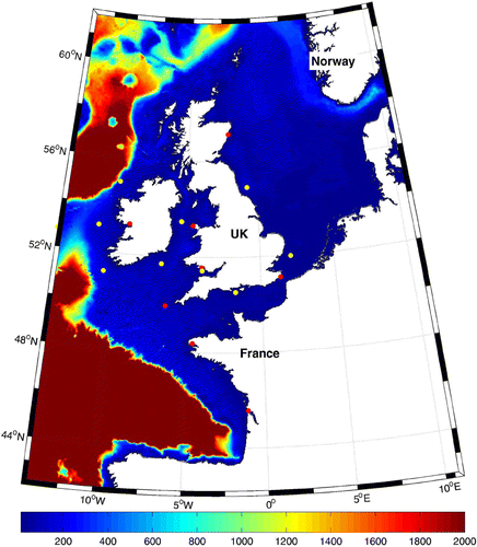
Table 2. The inter-monthly variability of wave energy during 2005–2011 averaged over the NW European shelf seas (the same study area as Neill and Hashemi (2013)).

Year	Jan	Feb	Mar	Apr	May	Jun	Jul	Aug	Sep	Oct	Nov	Dec
2005	74.2	35.2	21.9	21.2	11.8	8.3	9.0	12.0	18.3	29.9	42.9	29.2
2006	32.6	37.2	29.2	20.4	15.5	8.1	9.2	8.2	17.5	24.0	67.6	84.6
2007	65.4	54.2	50.6	11.0	19.7	10.3	9.9	13.5	19.5	15.9	26.6	56.7
2008	54.1	46.1	54.5	20.9	7.2	10.2	12.0	15.0	18.7	39.5	35.1	44.9
2009	72.8	25.7	35.2	16.1	21.2	8.4	12.2	14.1	18.9	26.0	71.7	39.8
2010	30.7	31.1	25.9	18.6	9.4	10.5	17.0	9.0	19.6	32.1	50.5	25.4
2011	23.6	72.2	30.6	28.4	23.6	13.6	12.0	11.2	23.9	35.4	47.2	77.3
Avg.	50.5	43.1	35.4	19.5	15.5	9.9	11.6	11.9	19.5	29.0	48.8	51.1
SD.	21.3	15.9	12.5	5.3	6.3	1.9	2.8	2.6	2.1	7.8	16.3	22.9
Min.	23.6	25.7	21.9	11.0	7.2	8.1	9.0	8.2	17.5	15.9	26.6	25.4
Max.	74.2	72.2	54.5	28.4	23.6	13.6	17.0	15.0	23.9	39.5	71.7	84.6

Figure 2. An example of a wave field generated in the North Atlantic Ocean and approaching the UK shelf seas. The colour scale (refer to the web version) represents the significant wave height in metres. The global wave data is extracted from the ECMWF ERA-Interim dataset.

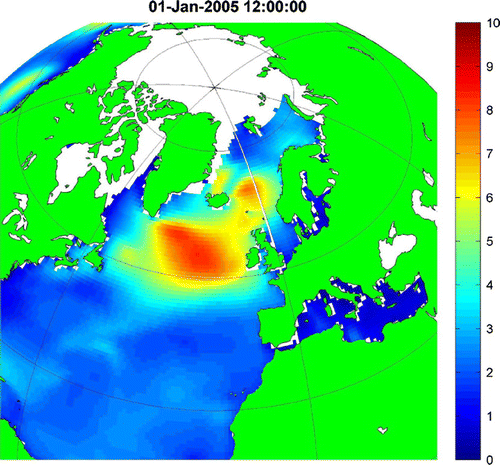
Figure 3. Validation of the ROMS results at a number of tidal gauges distributed across the domain. The absolute relative error for amplitude and phase of $M_2$ are 13 cm and $8^{\mathrm{o}}$, respectively. The corresponding values for $S_2$ amplitude and phase are 7 cm and ${11}^{\mathrm{o}}$. The locations of tidal gauges are reported in table 3.

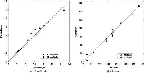
Figure 4. Comparison of the COAWST modelled amplitudes and FES2012 data. The axes units are metres.

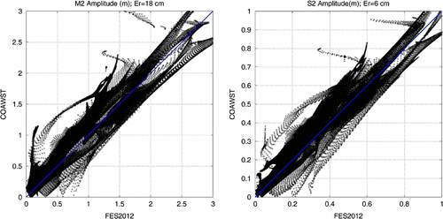
Figure 5. Cotidal charts of the main tidal constituents over the study area based on the ROMS model output. The colour scale (refer to the web version) indicates the amplitude while the phases are represented by the contour lines.

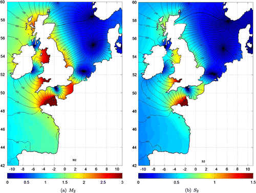
Figure 6. Tidal ellipses of the main tidal constituents representing the magnitude and direction of the tidal currents over the study area. The colour scale (refer to the web version) represents the velocity amplitude in m/s.

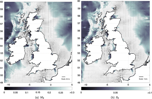
Figure 7. Validation of the COAWST wave height results at a number of wave buoys (table 3) during January 2005.

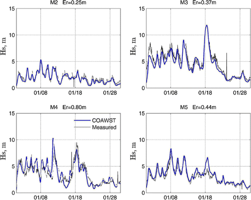
Figure 8. Validation of the COAWST wave period results at a number of wave buoys (table 3) during January 2005.

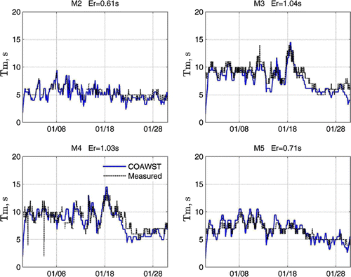
Table 3. Validation locations for COAWST tide and wave results.

Station	Coordinate
Mumbles, TG${}^{\mathrm{a}}$	3.97 W	51.57 N
St Marys, TG	6.32 W	49.93 N
Holyhead, TG	4.62 W	53.51 N
Aberdeen, TG	2.67 W	57.15 N
Dover, TG	1.32 E	51.07 N
Galway, TG	9.04 W	53.27 N
Pointe de Grave, TG	1.07 W	45.56 N
Brest, TG	4.50 W	48.38 N
M2, WB${}^{\mathrm{b}}$	5.43 W	53.48 N
M3, WB	10.55 W	51.22 N
M4, WB	9.99 W	54.99 N
M5, WB	6.70 W	51.69 N
Scarweather, WB	3.93 W	51.43 N
Poolebay, WB	1.72 W	50.63 N
West Gabbard, WB	2.08 E	51.98 N
Tynetees, WB	0.75 W	54.92 N

${}^{\mathrm{a}}$Tide Gauge ${}^{\mathrm{b}}$Wave Buoy

Figure 9. Validation of the COAWST wave height results at a number of wave buoys (table 3) during January–March 2007.

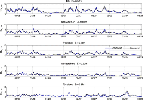
Figure 10. Validation of the COAWST wave period results at a number of wave buoys (table 3) during January–March 2007.

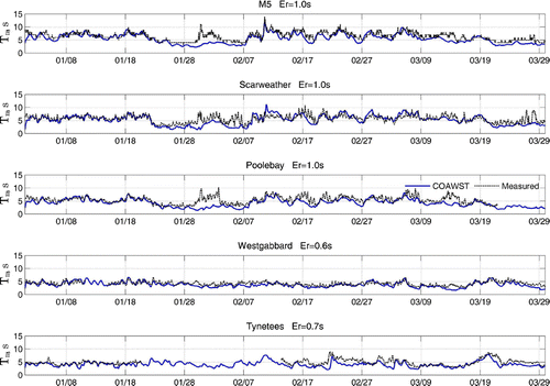
Figure 11. Comparison of the COAWST and decoupled-SWAN model performances in January 2007, at Scarweather wave buoy (table 3).

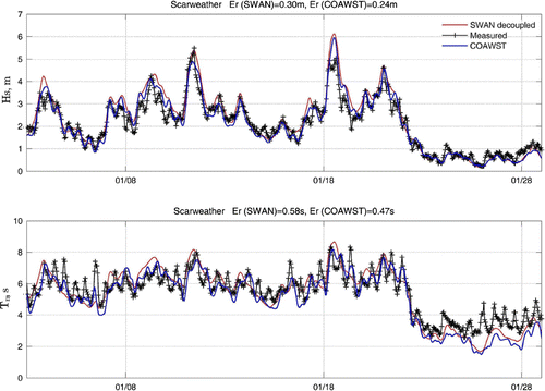
Table 4. Computational cost of decoupled ROMS and SWAN compared with COAWST for one month of simulation.

Model	Number of CPUs	Simulation time, h	Total cost, CPU-h
ROMS, Decoupled	96	3.32	319
SWAN, Decoupled	96	2.81	270
COAWST (ROMS + SWAN)	96 + 96	12.01	2304
COAWST (ROMS + SWAN (Nested))	96 + 96	12.03	2310

Figure 12. Computed average and maximum wave heights during January 2005 over the domain. The colour scale (refer to the web version) shows significant wave height in metres; (a) average and (b) maximum.

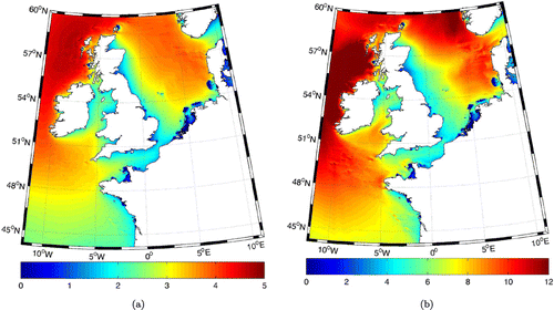
Figure 13. The average computed wave induced bottom stress (ignoring tide) and the average estimated bottom orbital velocities for January 2005 based on the COAWST results (refer to the web version for colour scales); (a) wave induced bottom stress ($\mathrm{N}/m^2$) and (b) estimated orbital velocities at the bed (m/s).

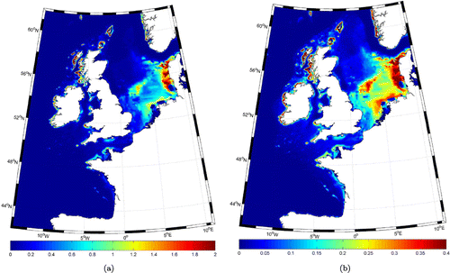
Figure 14. Average bed shear stress for January 2005, using the COAWST model for tidal current induced (ignoring waves) and combined wave-current induced cases. The colour scale (refer to the web version) is stress in $\mathrm{N}/m^2$; (a) tide induced bottom stress ($\mathrm{N}/m^2$) and (b) combined tide-wave induced bottom stress ($\mathrm{N}/m^2$).

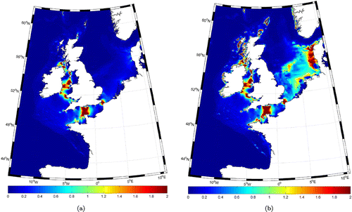
Figure 15. Effect of wave–tide interaction on the wave energy assessment for January 2005. The colour scale (refer to the web version) on the right hand plot represents the effect of tide on the wave power estimation in % which has been computed by subtracting the COAWST and decoupled SWAN model results. To avoid division by small numbers, the low-energy regions (less than 1/3 of the average) are filtered (set to green colour); (a) comparison of average wave power kW/m for January 2005, computed by different model configurations (fully coupled, one-way coupled, and uncoupled); and (b) effect of wave–tide interaction on the estimated wave power.

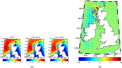
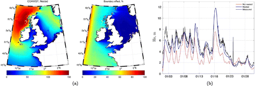
Figure 16. Effect of nesting on the computed wave parameters (refer to the web version for colour scales). The improvement of the model performance by nesting is significant, and over 30% in the west coasts of Ireland and Scotland. The effect is negligible in many parts of the Irish Sea and North Sea; (a) average wave power in January 2005 (left; kW/m) and effect of nesting on the results (right; %); and (b) effect of nesting on mode results at M3 wave buoy (see sub-figure a for location) in January 2005.

Neill, S.P. and Hashemi, M.R., Wave power variability over the northwest European shelf seas. App. Energ. 2013, 106, 31–46.

 Web of Science ®Google Scholar