Thin-jet scaling in large-scale shallow water quasigeostrophic flow

Figures & data

Figure 1. Potential vorticity field at t = 0 (left), t = 20, 000 (middle) and t = 50, 200 (right). (Colour online).

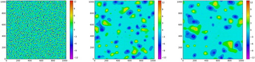
Figure 2. Kinetic energy density at t = 0 (left), t = 20, 000 (middle) and $t=50,200$ (right). (Colour online).

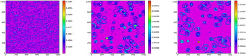
Figure 3. Potential vorticity field (left) and kinetic energy density at $t=403,000$ (right). (Colour online).

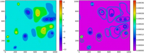
Figure 4. Left: typical area $A_{\mathrm{t}\mathrm{y}\mathrm{p}}^{\mathrm{e}\mathrm{x}\mathrm{t}}$ of mixed regions bounded by external fronts (black squares) with least squares best fit line (solid black), typical area $A_{\mathrm{t}\mathrm{y}\mathrm{p}}$ (violet triangles) with best fit line (dashed violet), typical area $A_{\mathrm{t}\mathrm{y}\mathrm{p}}^{\mathrm{i}\mathrm{n}\mathrm{t}}$ of mixed regions bounded by internal fronts (blue asterisks) with best fit line (dash-dot blue), and typical area $A_{\mathrm{t}\mathrm{y}\mathrm{p}}^{\mathrm{f}\mathrm{r}\mathrm{e}\mathrm{e}}$ regions within free vortex cores (magenta circles), with best fit line (magenta dotted). Right: number of mixed regions bounded by external fronts (black squares) with least squares best fit line (solid black), mixed regions bounded by internal fronts (blue asterisks) with best fit line (dash-dot blue), and regions within free vortex cores (magenta circles). (Colour online).

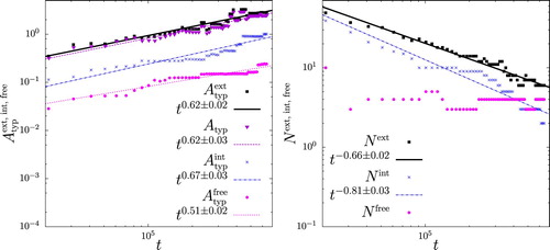
Figure 5. Results of the mixed region and free vortex core extractions (left) and high-speed contour extractions (right) at t = 403, 000. Regions bounded by external fronts, internal fronts and contained within free vortex cores are shown in the top, middle and bottom left panels, respectively, while the corresponding bounding contours composing the external PV fronts, internal PV fronts and boundaries of the free cores are shown in the top, middle and bottom right, respectively. (Colour online).

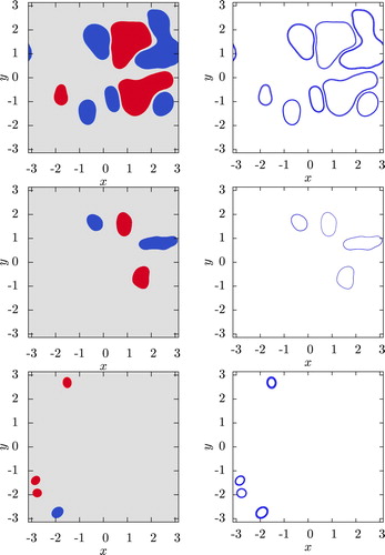
Table 1. Thresholds for the extraction of mixed regions.

Mixed region type	$q_{\mathrm{t}\mathrm{h}\mathrm{r}}$	$A_{\mathrm{t}\mathrm{h}\mathrm{r}}^{\mathrm{m}\mathrm{i}\mathrm{n}}$	$A_{\mathrm{t}\mathrm{h}\mathrm{r}}^{\mathrm{m}\mathrm{a}\mathrm{x}}$
External	$0.25q_{\mathrm{r}\mathrm{m}\mathrm{s}}$	$A_{\mathrm{t}\mathrm{y}\mathrm{p}}/9$	–
Internal	$1.7q_{\mathrm{r}\mathrm{m}\mathrm{s}}\phantom{1}$	$A_{\mathrm{t}\mathrm{y}\mathrm{p}}/9$	–
Free core	$0.25q_{\mathrm{r}\mathrm{m}\mathrm{s}}$	$4\pi L_D^2$	$A_{\mathrm{t}\mathrm{y}\mathrm{p}}/9$

Note: The PV on the region must exceed $q_{\mathrm{t}\mathrm{h}\mathrm{r}}$, while the area of the region must be greater than $A_{\mathrm{t}\mathrm{h}\mathrm{r}}^{\mathrm{m}\mathrm{i}\mathrm{n}}$ and smaller than $A_{\mathrm{t}\mathrm{h}\mathrm{r}}^{\mathrm{m}\mathrm{a}\mathrm{x}}$.

Table 2. Thresholds for the extraction of high-speed frontal contours.

Contour type	$q_{\mathrm{t}\mathrm{h}\mathrm{r}}^{\mathrm{m}\mathrm{i}\mathrm{n}}$	$q_{\mathrm{t}\mathrm{h}\mathrm{r}}^{\mathrm{m}\mathrm{a}\mathrm{x}}$	$L_{\mathrm{t}\mathrm{h}\mathrm{r}}^{\mathrm{m}\mathrm{i}\mathrm{n}}$	$L_{\mathrm{t}\mathrm{h}\mathrm{r}}^{\mathrm{m}\mathrm{a}\mathrm{x}}$	${\overline{u}}_{\mathrm{t}\mathrm{h}\mathrm{r}}$
External	$0.25q_{\mathrm{r}\mathrm{m}\mathrm{s}}$	$1.3q_{\mathrm{r}\mathrm{m}\mathrm{s}}$	$L_{\mathrm{t}\mathrm{y}\mathrm{p}}/3$	–	$u_{\mathrm{r}\mathrm{m}\mathrm{s}}/4$
Internal	$1.7q_{\mathrm{r}\mathrm{m}\mathrm{s}}\phantom{1}$	$2q_{\mathrm{r}\mathrm{m}\mathrm{s}}\phantom{.1}$	$L_{\mathrm{t}\mathrm{y}\mathrm{p}}/3$	–	$u_{\mathrm{r}\mathrm{m}\mathrm{s}}/4$
Free core	$0.25q_{\mathrm{r}\mathrm{m}\mathrm{s}}$	$1.3q_{\mathrm{r}\mathrm{m}\mathrm{s}}$	$4\pi L_D$	$L_{\mathrm{t}\mathrm{y}\mathrm{p}}/3$	$u_{\mathrm{r}\mathrm{m}\mathrm{s}}/4$

Note: The PV on the region must exceed $q_{\mathrm{t}\mathrm{h}\mathrm{r}}^{\mathrm{m}\mathrm{i}\mathrm{n}}$ and be less than $q_{\mathrm{t}\mathrm{h}\mathrm{r}}^{\mathrm{m}\mathrm{a}\mathrm{x}}$, while the length of the contour must be greater than $L_{\mathrm{t}\mathrm{h}\mathrm{r}}^{\mathrm{m}\mathrm{i}\mathrm{n}}$ and less than $L_{\mathrm{t}\mathrm{h}\mathrm{r}}^{\mathrm{m}\mathrm{a}\mathrm{x}}$, and the average along-contour speed must exceed ${\overline{u}}_{\mathrm{t}\mathrm{h}\mathrm{r}}$.

Figure 6. Total contour length $L_{\mathrm{t}\mathrm{o}\mathrm{t}}$ (open blue circles), rms curvature ${\kappa }_{\mathrm{r}\mathrm{m}\mathrm{s}}$ (open red squares), and fluctuation curvature ${\kappa }_{\mathrm{f}\mathrm{l}}$ (filled black triangles) for high-speed contours comprising external (left) and internal (right) fronts. Least squares best fit lines are also shown for ${\kappa }_{\mathrm{r}\mathrm{m}\mathrm{s}}$ (cyan), $L_{\mathrm{t}\mathrm{o}\mathrm{t}}$ (magenta) and ${\kappa }_{\mathrm{f}\mathrm{l}}$ (black). The uncertainty given is the standard error. (Colour online).

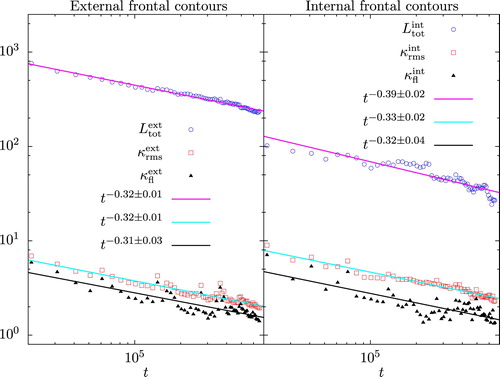
Figure 7. Disturbed PV contours undergoing filamentation after a merger at $t=140,000$. The area within the rectangle in the top panel is shown in the bottom panel: the inner two contours (blue and magenta) are undergoing filamentation. (Colour online).

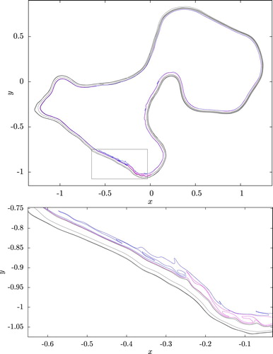
Figure 8. External bounding contours undergoing a reconnection and split. The time is given at the top of each panel. (Colour online).

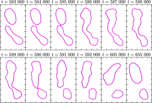
Figure 9. Total arclength (top), enclosed area (middle) and area between contours (bottom) for the contours shown in figure 8. (Colour online).

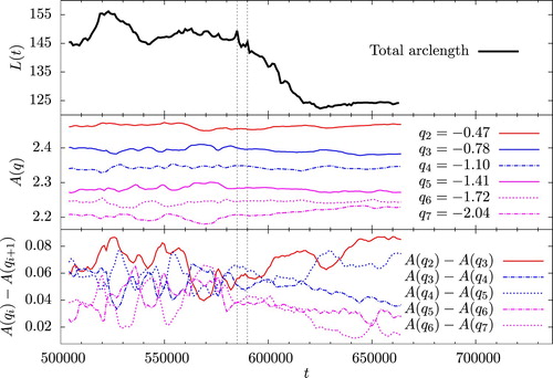
Figure 10. Total contour length $L_{\mathrm{t}\mathrm{o}\mathrm{t}}$ (open blue circles), rms curvature ${\kappa }_{\mathrm{r}\mathrm{m}\mathrm{s}}$ (open red squares), and fluctuation curvature ${\kappa }_{\mathrm{f}\mathrm{l}}$ (solid black triangles) for high-speed contours bounding free vortex cores. (Colour online).

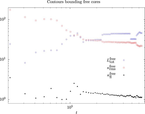
Figure 11. Check of the population-averaged relation (28(28) $\frac{1}{N_{\mathrm{c}\mathrm{o}\mathrm{n}\mathrm{t}}}\sum _j\left[\int {\kappa }_j^2\mathrm{d}s-\int ({\kappa }_j-{\overline{\kappa }}_j{)}^2\mathrm{d}s\right]=⟨\frac{4{\pi }^2}{L}⟩,$(28) ). (Colour online).

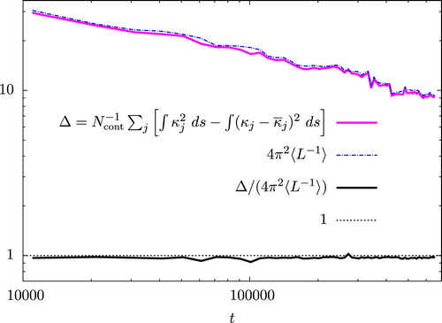
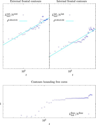
Figure 12. Average arc length of internal frontal contours (top left), external frontal contours (top right) and contours bounding free vortex cores (bottom). Least squares best fit lines (cyan) are also shown for the internal and external frontal contours. (Colour online).