Instabilities and vertical mixing in river plumes: application to the Bay of Biscay

Figures & data

Figure 1. Suspended matters for top row: (left) Winter, (right) Spring and bottom row: (left) Summer and (right) Fall. The quarterly climatology is based on MERIS/ESA and MODIS/NASA data from 2003 to 2013, following the approach developed in Gohin (2011) and processed in the MARC project (http://marc.ifremer.fr/). Location of Le Verdon MAGEST in situ observing network station in the Gironde estuary (blue point – top left).

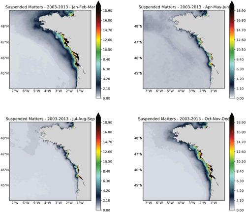
Figure 2. Bathymetry of the idealised numerical model configuration. (Colour online)

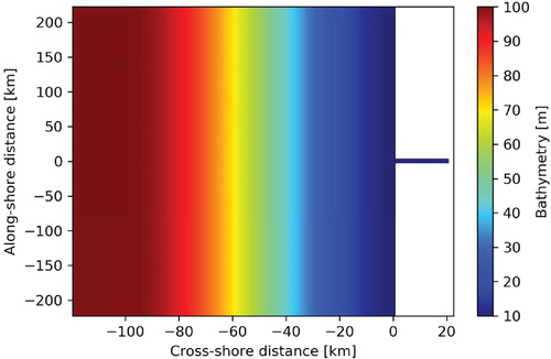
Figure 3. Le Verdon MAGEST station time series of salinity at $\sim 1\mathrm{m}$ depth during January and February 2019. The black dashed line shows the 20 psu salinity value used for idealised simulations. (Colour online)

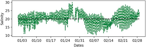
Figure 4. The Gironde estuary is fed by the Garonne and Dordogne rivers. The discharges for these two rivers are obtained from hydrological stations and retrieved through the French national service “Banque Hydro” (https://www.hydro.eaufrance.fr). They are added together to estimate the Gironde discharge. Blue dots show the monthly discharge mean. For each month, the standard deviation of the river discharge is represented by a vertical bar. The red dashed line shows the $1550{\mathrm{m}}^3{\mathrm{s}}^{-1}$ discharge value used in idealised simulations. (Colour online)

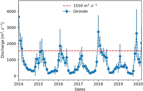
Table 1. List of simulations and their specific forcings.

Experiments	River forcing	External forcings
Reference	Discharge ($1550{\mathrm{m}}^3{\mathrm{s}}^{-1}$)	–
High Discharge	Discharge ($\mathrm{10,000}{\mathrm{m}}^3{\mathrm{s}}^{-1}$)	–
Tide	Discharge ($1550{\mathrm{m}}^3{\mathrm{s}}^{-1}$)	M2 Tide (1.5 m amplitude)
Wind	Discharge ($1550{\mathrm{m}}^3{\mathrm{s}}^{-1}$)	SW Wind (${\tau }_{max}=0.02\mathrm{N}{\mathrm{m}}^{-2}$)

Figure 5. Sea Surface Salinity at three different time steps – Reference Configuration. The black dashed line represents zonal vertical sections shown hereafter. The bold black rectangle represents the bulge region. The bold dashed rectangle defines the coastal current. (Colour online)

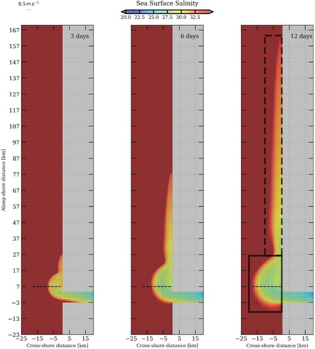
Figure 6. Vertical sections of Potential density (day 12): (a) Reference, (b) High Discharge, (c) Tide, (d) SW wind. The black dashed line represents the vertical profiles (density and $N^2$) shown hereafter. (Colour online)

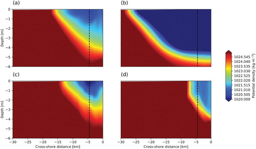
Figure 7. Brunt–Vaisala (left) and potential density (right) vertical profiles (12 day). (Colour online)

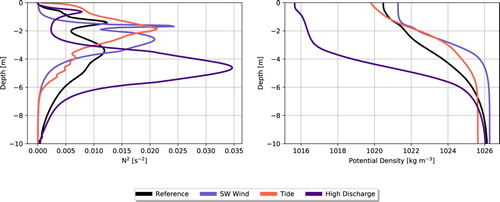
Figure 8. Surface scaled relative vorticity (day 12): (a) Reference, (b) High Discharge, (c) Tide, (d) SW wind. (Colour online)

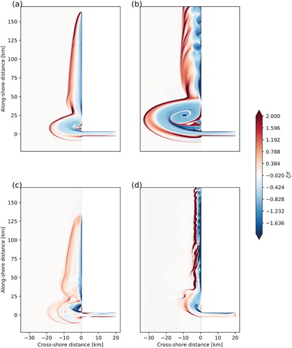
Figure 9. Vertical sections of scaled relative vorticity (day 12): (a) Reference, (b) High Discharge, (c) Tide, (d) SW wind. (Colour online)

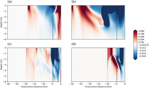
Figure 10. KE density spectrum at the surface (left) and at the river plume base (right). (Colour online)

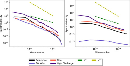
Figure 11. Sea surface salinity at three different time steps – high discharge configuration. The black dashed line represents zonal vertical sections shown hereafter. (Colour online)

Figure 12. Sea surface salinity at three different time steps – SW Wind Configuration. The black dashed line represents zonal vertical sections shown hereafter. (Colour online)

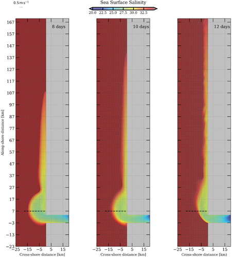
Figure 13. Sea surface salinity at three different time steps – Tide Configuration. The black dashed line represents zonal vertical sections shown hereafter. (Colour online)

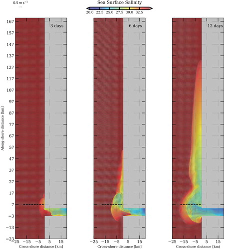
Figure 14. $f{\mathrm{\partial }}_{x}Q$ at the river plume base (day 12) for (a) Reference, (b) High Discharge, (c) Tide, (d) SW wind. (Colour online)

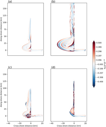
Figure 15. Vertical section $f{\mathrm{\partial }}_{x}Q$ (day 12) for (a) Reference, (b) High Discharge, (c) Tide, (d) SW wind. (Colour online)

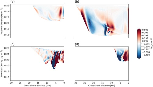
Figure 16. fQ at the river plume base (day 12) for (a) Reference, (b) High discharge, (c) Tide, (d) SW wind. (Colour online)

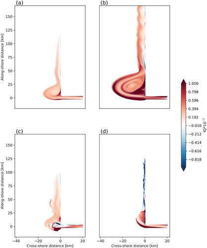
Figure 17. Richardson number at the river plume base (day 12) for (a) Reference, (b) High discharge, (c) Tide, (d) SW wind. (Colour online)

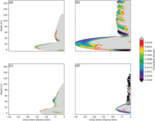
Figure 18. Integrated (from river plume base to surface – day 10) HRS (left),VBF (middle) and VRS (right) for the reference configuration. (Colour online)

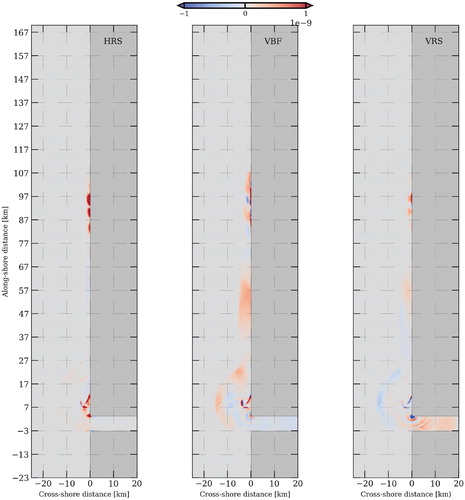
Figure 19. Vertical sections (isopycnes) fQ (day 12) for (a) Reference, (b) High Discharge, (c) Tide, (d) SW wind. (Colour online)

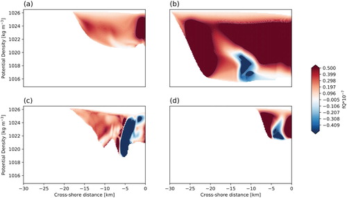
Figure 20. Vertical section Richardson Number (day 12) for (a) Reference, (b) High Discharge, (c) Tide, (d) SW wind. The black solid contour indicates the critical Richardson number $R{i}_c=0.25$. (Colour online)

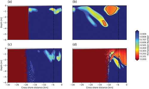
Figure 21. Integrated (from river plume base to surface – day 10) HRS (left),VBF (middle) and VRS (right) for the high discharge configuration. (Colour online)

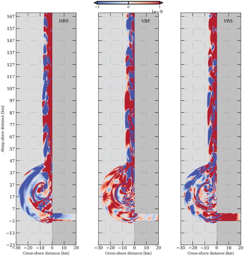
Figure 22. Integrated (from river plume base to surface – day 10) HRS (left),VBF (middle) and VRS (right) for the SW wind configuration. (Colour online)

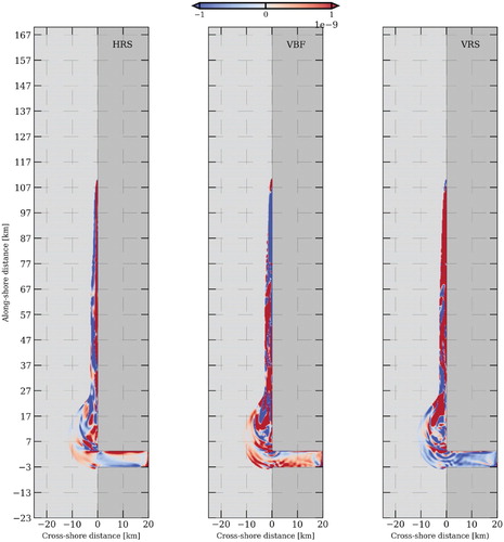
Figure 23. Integrated (from river plume base to surface – day 10) HRS (left),VBF (middle) and VRS (right) for the Tide configuration. (Colour online)

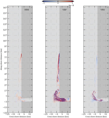
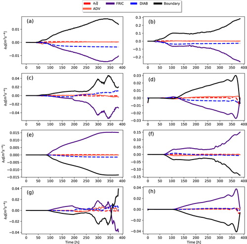
Figure 24. Stratification,frontogenesis and PV anomaly for (a) the Reference, (b) High discharge, (c) SW wind, (d) M2 Tide configurations in the bulge and (e–h) same configurations in the coastal current. (Colour online)

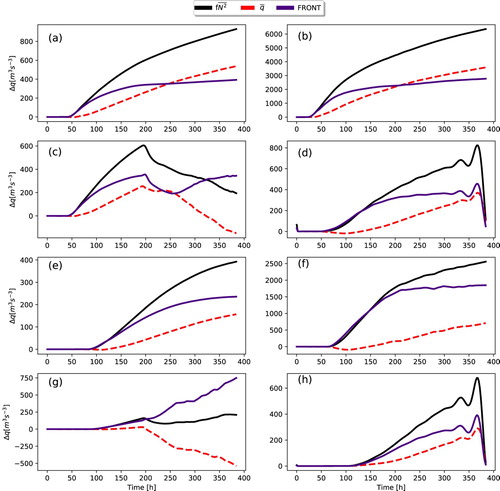
Figure 25. Pv flux terms for (a) the Reference, (b) High discharge, (c) SW wind, (d) M2 Tide configurations in the bulge and for (e–h) same configurations in the coastal current. (Colour online)

Gohin, F., Annual cycles of chlorophyll-a, non-algal suspended particulatematter, and turbidity observed from space and in-situ incoastal waters. Ocean Sci. 2011, 7, 705–732.

 Web of Science ®Google Scholar