Formation of small-scale vortices in the core of a large merged vortex

Figures & data

Figure 1. Series of temperature maps in the $(x,y)$-plane at t = 0, 3, 4.5, 9, 12, 15 illustrating the formation of a row of small vortices at the centre of the merged vortex for $d/R=2.5$ at resolution $1024\times 1024$. The black lines denote the contours of various temperature levels between 0 and 1. (a) t = 0.0. (b) t = 3.0. (c) t = 4.5. (d) t = 9. (e) t = 12 and (f) t = 15.

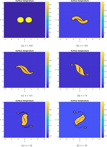
Figure 2. Okubo-Weiss quantity OW (left panel) and frontogenetic function FGT map (right panel) in the $(x,y)$-plane at time t = 3 illustrating the deformation of the internal front for $d/R=2.5$ at resolution $1024\times 1024$. The black lines in the left hand panel are the contours of the various levels of the Okubo-Weiss parameter between 0 and the maximal positive or negative values. (a) OW – t = 3.0 and (b) FGT – t = 3.0 (Colour online).

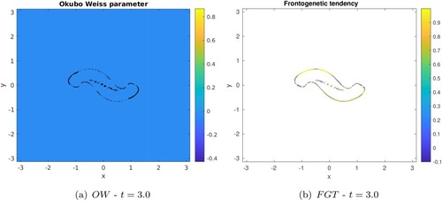
Figure 3. Evolution of the passive tracer distribution in the $(x,y)$-plane from left to right then top to bottom at time t = 0, 1.5, 3.0, 4.5 for $d/R=2.5$ at resolution $1024\times 1024$. The black lines denote the various levels of tracer concentration; their closeness indicates a locally strong tracer gradient. (a) t = 0.0. (b) t = 2.5. (c) t = 3.50 and (d) t = 4.5 (Colour online).

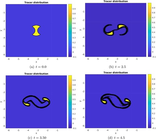
Figure 4. Evolution of the temperature in the $(x,y)$-plane at time t = 3.0, 4.5 for top-hat vortices with $d/R=2.0$ (top row), at time t = 4.5, 6.0 for top-hat vortices with $d/R=2.8$ (middle row), at time t = 6.0, 7.5 for smooth vortices with $d/R=2.3$ (bottom row). These simulations were performed at $1024\times 1024$ resolution. The black lines are the contours of the various levels of temperature in the model. Their closeness indicates a high gradient of temperature. (a) t = 3.0. (b) t = 4.5. (c) t = 4.5. (d) t = 6.0. (e) t = 6.0 and (f) t = 7.5.

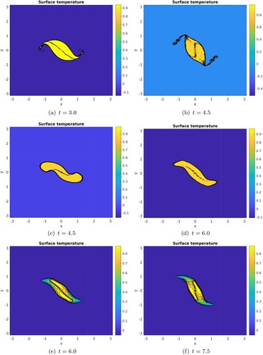
Figure 5. Meridional section of the temperature distribution in the parallel strip under study.

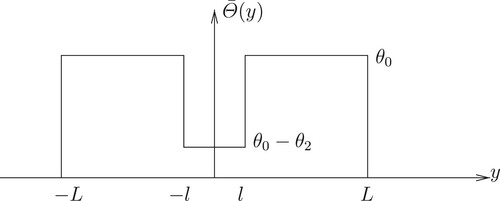
Figure 6. Horizontal structure of the temperature distribution in the perturbed parallel gaped strip.

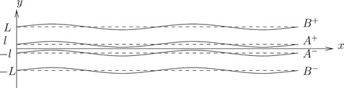
Figure 7. Growth rates of linear perturbation on the mean temperature profile; the growth rates are displayed in the $(kL,l/L)$-plane for $U_2^{\ast }/U_0^{\ast }=0.1,0.5,0.9$ (left column) and in the (kL, $U_2^{\ast }/U_0^{\ast }$)-plane for $l/L=0.1,0.5,0.9$ (right column).

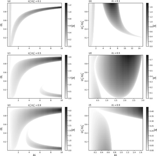
Figure 8. Nonlinear evolution of the unstable parallel temperature distribution with $l/L=0.1,U_2^{\ast }/U_0^{\ast }=1.0$, perturbed with a white noise in temperature with amplitude 0.1 initially, at time t = 0, 8.0, 16.0, 20.0, 24.0 (from left to right and from top to bottom). The lower left plot is a zoom on the central vortex for the last subplot. These simulations were performed at $1024\times 1024$ resolution. The black lines are the various contours of temperature. Their closeness denotes a high gradient of temperature, in particular in the filaments. (a) t = 0.1. (b) t = 8.0. (c) t = 16.0. (d) t = 20.0. (e) t = 24.0 and (f) t = 24.0 – zoom.

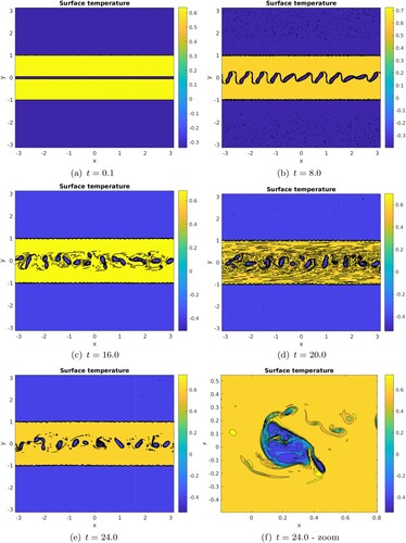
Figure 9. Modal analysis ($A_m$ is the amplitude of the zonal mode with wavenumber m) for the unstable parallel temperature distribution with $l/L=0.1,U_2^{\ast }/U_0^{\ast }=1.0$ presented in figure 8.

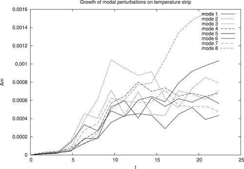
Figure 10. Zoom on the central region of figure 1 at time t = 6.0 and t = 9.0; row of small vortices in the core of the large merged vortex. The black lines indicate the various levels of surface temperature, separating the various colours. (a) t = 6.0 and (b) t = 9.0 (Colour online).

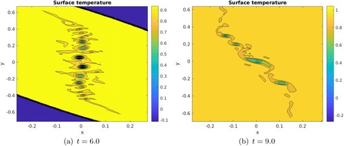
Figure 11. Time evolution of horizontal maps of temperature using the nonlinear spectral SQG model. Times shown are t = 0, 5, 35, 40. The simulation is initialised with 6 small vortices along the major axis of a 2:1 large elliptical vortex. The small vortices have the following radius and separation $R_1=0.1,d^{\prime }=0.25$. This simulation was performed at $1024\times 1024$ resolution. The black lines indicate the various contours of temperature. The temperature gradients are large in the filaments and at the vortex peripheries. (a) t = 0.0. (b) t = 5.0. (c) t = 35.0 and (d) t = 40.0 (Colour online).

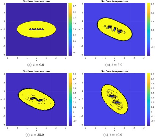
Figure 12. Evolution of horizontal maps of passive tracer for an ellipse without (top) or with (bottom) small central vortices. Times shown are t = 0, 16, 32. The second simulation is initialised with 6 small vortices along the major axis of a 2:1 large elliptical vortex. The small vortices have the following radius and separation $R_1=0.1,d=0.25$. The resolution of this simulation is $1024\times 1024$. The black lines indicate the various levels of tracer concentration. (a) t = 0.0. (b) t = 16.0. (c) t = 32.0. (d) t = 0.0. (e) t = 16.0 and (f) t = 32.0 (Colour online).

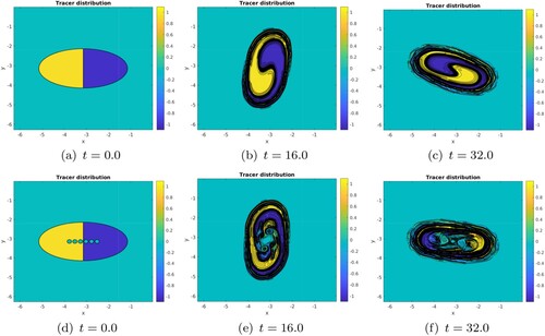
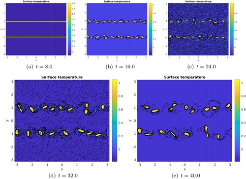
Figure A1. Nonlinear evolution of the unstable parallel temperature distribution with $l/L=0.5,U_2^{\ast }/U_0^{\ast }=1.0$, perturbed with a white noise in temperature with amplitude 0.1 initially, at time t = 0, 12.8, 25.6, 38.4. The black lines indicate the various levels of surface temperature. (a) t = 0.0. (b) t = 12.8. (c) t = 25.6 and (d) t = 38.4 (Colour online).

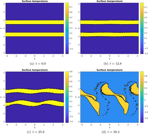
Figure A2. Nonlinear evolution of the unstable parallel temperature distribution with $l/L=0.9,U_2^{\ast }/U_0^{\ast }=1.0$, perturbed with a white noise in temperature with amplitude 0.1 initially, at time t = 0, 8.0, 16.0, 24.0, 32.0, 40.0. The black lines indicate the various levels of surface temperature. (a) t = 8.0. (b) t = 16.0. (c) t = 24.0. (d) t = 32.0 and (e) t = 40.0 (Colour online).