A study of global magnetic helicity in self-consistent spherical dynamos

Figures & data

Table 1. The three dynamo solutions considered in the study.

	Case 1: Steady dynamo	Case 2: Quasi-periodically reversing dynamo	Case 3: Aperiodically-reversing dynamo
η	0.35	0.4	0.4
$R_i$	0	3.5 $\times {10}^6$	$8.5\times {10}^5$
$R_e$	${10}^5$	0	0
τ	2000	$3\times {10}^4$	$3\times {10}^4$
P	1	0.75	0.1
$P_m$	5	0.65	1
Boundary conditions	no-slip, fixed temperatures, insulating outer space	stress-free, fixed temperatures, insulating outer space	stress-free, fixed temperatures, insulating outer space

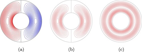
Figure 1. Plots of the velocity field for Case 1 at a particular time (this is a steady flow so other times just represent rigid rotations of this solution) (a) shows lines of constant ${\overline{u}}_{\varphi }$ (left half) and $r\sin \theta {\mathrm{\partial }}_{\theta }\overline{v}$ (right half) in a meridional plane, visualising the toroidal and poloidal fields respectively; (b) shows lines of constant $u_r$ at $r=r_i+0.5$. There is a distinct pattern of columnar convection at both the equator and near the poles; and (c) shows lines of constant $r{\mathrm{\partial }}_{\varphi }v$ in the equatorial plane. Blue is negative, red is positive and green is zero in this figure and in all subsequent contour plots. (Colour online).

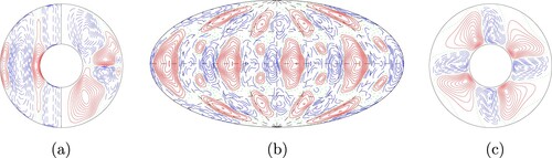
Figure 2. Plots of the magnetic field (top row) and magnetic helicity (bottom row) for Case 1 at a particular time. The top panel (a) shows meridional lines of constant ${\overline{B}}_{\varphi }$ (left half) and $r\sin \theta {\mathrm{\partial }}_{\theta }\overline{h}$ (right half) visualising the toroidal and poloidal fields respectively; (b) shows lines of constant $B_r$ at $r=r_i+0.96$; and (c) displays equatorial streamlines, $r{\mathrm{\partial }}_{\varphi }h$ = const. The bottom panel (d) shows contour lines of azimuthally averaged helicity density (left half) and the helicity density in a particular slice $\varphi =\mathrm{c}\mathrm{o}\mathrm{n}\mathrm{s}\mathrm{t}$ (right half); (e) shows the helicity density at $r=r_i+0.96$; and (f) shows the helicity density at the equatorial plane.

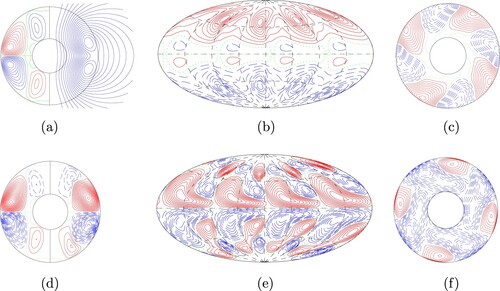
Figure 3. A representation of the linkage of toroidal and poloidal fields. Colours correspond to those in figure 2(a). The (Gauss) linkage in (a) is $-1$ and in (b) is $+1$. These signs correspond with those of the helicity density in figure 2(d). (Colour online).

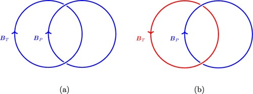
Figure 4. Typical structures of the velocity field for Case 2. (a) shows lines of constant ${\overline{u}}_{\varphi }$ in the left half and streamlines $r\sin \theta {\mathrm{\partial }}_{\theta }\overline{v}$ = const in the right half, all in the meridional plane; (b) shows lines of constant $u_r$ at $r=r_i+0.5$; and (c) shows streamlines, $r{\mathrm{\partial }}_{\varphi }v$ = const. in the equatorial plane. These images correspond to the time t = 5.538 in the simulation. (Colour online).

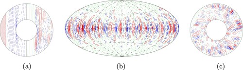
Figure 5. Time series of magnetic helicity for Case 2. (a) shows the total helicity as a function of time. (b) shows the helicity density integrated in the northern hemisphere (solid) and the southern hemisphere (dashed).

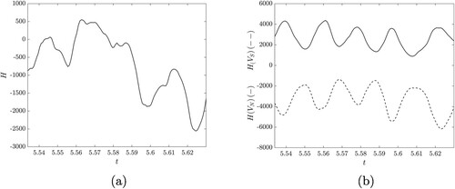
Figure 6. Time series related to reversals. (a) displays reversals of the poloidal and toroidal fields. The poloidal and toroidal fields are represented by their dominant spectral expansion components $H_1^0$ (solid line) and $G_1^0$ (dashed line), respectively. Both of these quantities are calculated at $r=r_i+0.5$. (b) displays the total magnetic energy $E_B$, which oscillates at a frequency similar to the hemispheric helicities displayed in figure 5.

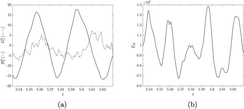
Figure 7. A latitude vs time plot of the magnetic helicity density at the surface for Case 2 with a nonlinear colourmap: indigo (−400, −30); maroon (−30, 30) and seismic (blue and red) (30, 400).

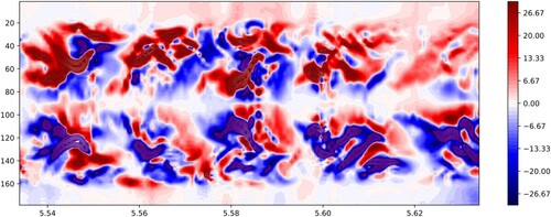
Figure 8. Typical structures of the velocity field in the case. (a) shows lines of constant ${\overline{u}}_{\varphi }$ in the left half and streamlines $r\sin \theta {\mathrm{\partial }}_{\theta }\overline{v}$ = const. in the right half, all in the meridional plane; (b) shows lines of constant $u_r$ at $r=r_i+0.5$ and (c) shows streamlines, $r{\mathrm{\partial }}_{\varphi }v$ = const. in the equatorial plane. These images correspond to the time t = 13.52 in the simulation.

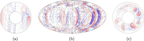
Figure 9. Time series during a reversal. $H_1^0$ (solid) and $G_1^0$ (dashed) are displayed in (a). Both quantities are evaluated at $r=r_i+0.5$. The blue vertical lines indicate the reversal times of these quantities. The northern (solid) and southern (dashed) helicities are shown in (b). Reversal times are indicated by green vertical lines. Just before the final green line, there are very small reversals about the H = 0 axis, and these are not shown. (Colour online).

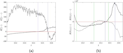
Table 2. The helicity and magnetic field reversal times for the other observed reversals.

Reversals	$H_1^0$	$G_1^0$	$H\left(V_N\right)$	$H\left(V_S\right)$	$H\left(V_N\right)$ and $H\left(V_S\right)$
2	26.3232	26.374	26.199	26.3313	26.3504
3	31.2784	31.3534	31.169	31.2532	31.3047

Figure 10. A latitude vs time plot of the magnetic helicity density at the surface for Case 3 with a nonlinear colourmap: indigo (−500, −30); maroon (−30, 30; shown) and seismic (blue and red) (30, 500).

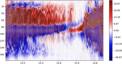
Figure A1. (a) shows meridional lines of constant ${\overline{B}}_{\varphi }$ (left half) and $r\sin \theta {\mathrm{\partial }}_{\theta }\overline{h}$ (right half); (b) shows averaged helicity density (left half) and unaveraged helicity density (right half); (c) shows the helicity density in the equatorial plane. (Colour online).