Resonant growth of inertial oscillations from lee waves in the deep ocean

Figures & data

Figure 1. Numerical setting. A uniform geostrophic current $U_G$ flows over a sinusoidal topography of horizontal wavenumber $k_T$ and height 2H in a two-dimensional domain with horizontal periodic boundary conditions. Internal lee waves are emitted, as sketched by dashed phase lines, which are damped in a sponge layer of thickness 5000 m starting at 2000 m above topography.

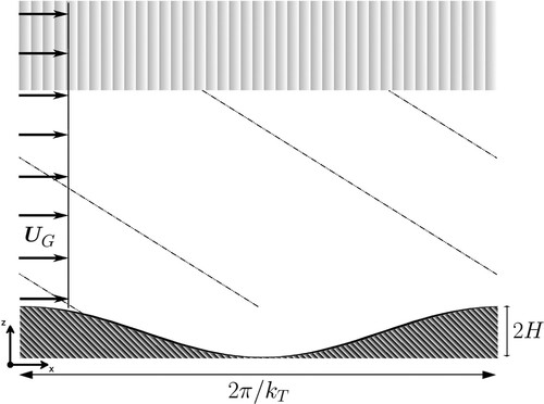
Table 1. Summary of the simulations.

Simulation	L	H	f	Bottom condition	$U_G/NH$
$H_{20}{L}_2$	$2\mathrm{km}$	20 m	${1.10}^{-4}$ s${}^{-1}$	Partial-slip	5
$H_{40}{L}_2$	$2\mathrm{km}$	40 m	${1.10}^{-4}$ s${}^{-1}$	Partial-slip	2.5
$H_{80}{L}_2$	$2\mathrm{km}$	80 m	${1.10}^{-4}$ s${}^{-1}$	Partial-slip	1.25
$H_{20}{L}_2\mathrm{\_}fs$	$2\mathrm{km}$	20 m	${1.10}^{-4}$ s${}^{-1}$	Free-slip
$H_{40}{L}_2\mathrm{\_}fs$	$2\mathrm{km}$	40 m	${1.10}^{-4}$ s${}^{-1}$	Free-slip
$H_{80}{L}_2\mathrm{\_}fs$	$2\mathrm{km}$	80 m	${1.10}^{-4}$ s${}^{-1}$	Free-slip
$H_{20}{L}_{1.2}$	$1.2\mathrm{km}$	20 m	${1.10}^{-4}$ s${}^{-1}$	Partial-slip
$H_{40}{L}_{1.2}$	$1.2\mathrm{km}$	40 m	${1.10}^{-4}$ s${}^{-1}$	Partial-slip
$H_{80}{L}_{1.2}$	$1.2\mathrm{km}$	80 m	${1.10}^{-4}$ s${}^{-1}$	Partial-slip
$H_{40}{L}_2\mathrm{\_}2f$	$2\mathrm{km}$	40 m	${2.10}^{-4}$ s${}^{-1}$	Partial-slip
$H_{80}{L}_2\mathrm{\_}2f$	$2\mathrm{km}$	80 m	${2.10}^{-4}$ s${}^{-1}$	Partial-slip

Notes: L is the horizontal length of the numerical domain (equal to the horizontal wavelength of the topography), H is the half-height of the topography and f is the Coriolis parameter. Either partial-slip or free-slip boundary conditions are used at the topography for the velocity field. The other physical and numerical parameters are the same for all simulations and described in section 2.

Figure 2. Snapshots of the vertical velocity for simulation $H_{40}{L}_2$ after one inertial period (upper frame) and after 7 inertial periods (lower frame). The same colorbar is used for the two frames, but the maximum value is about three times higher in the lower than in the upper frame. Note the quasi-linear regime in the upper frame and the strongly nonlinear regime in the lower one.

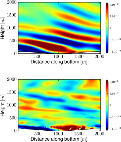
Figure 3. Temporal evolution of the inertial oscillation (IO) amplitude at about 10 m above the topography top, as a function of time scaled by the inertial period $2\pi /f$. The IO signal was processed through a Lanczos low-pass filter at cutoff frequency f. The spin-up of the simulation, during which the geostrophic current grows from 0 to the value of $U_G$, is not shown (Colour online).

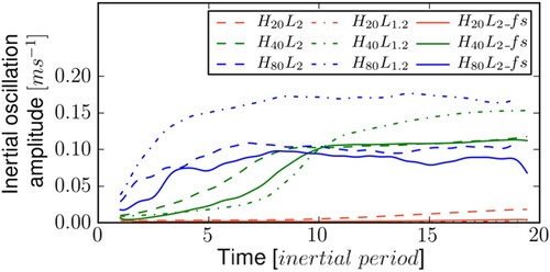
Figure 4. Vertical structure of the IO horizontal velocity (upper frame) and of the horizontally-averaged TKE dissipation rate (lower frame) for the simulations displayed in table 1. All fields are averaged from 12 to 15 inertial periods (Colour online).

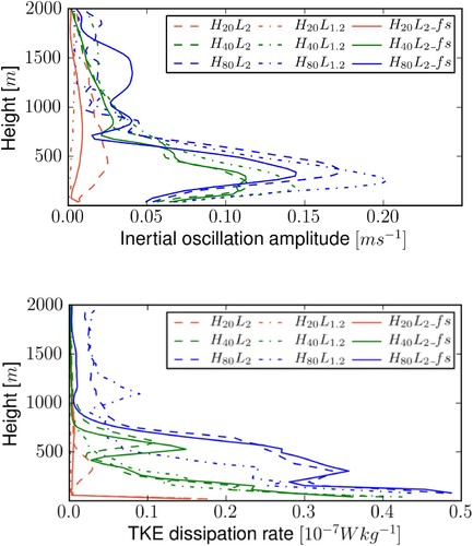
Figure 5. Variance preserving power spectrum of the horizontal velocity component of the wave field for simulation $H_{20}{L}_2$ computed at about 600 m above the bottom of the domain, in a frame of reference moving with the geostrophic velocity $U_G$. The wave field encompasses the entire flow, except for the geostrophic flow. The straight line is the confidence level at 99% implying that the spectrum significantly departs from red noise when it exceeds this line. The inertial and buoyancy frequencies and the frequencies predicted by the resonant interaction theory are indicated with a vertical dashed-dotted line. The length of the time series is 15 inertial periods implying that the spectral resolution is 0.01f.

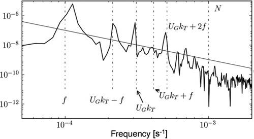
Figure 6. Scatter diagram of the growth rate of the IO diagnosed from the simulations, ${\Gamma }_{sim}$, versus that computed from the resonant interaction theory, ${\Gamma }_{RIT}$, scaled by the inertial frequency. Simulations for which the inverse of the IO growth rate is smaller than 3 inertial periods are indicated with a filled marker (black or grey). For simulations with empty markers, the inverse of the IO growth rate is larger than 10 inertial periods.

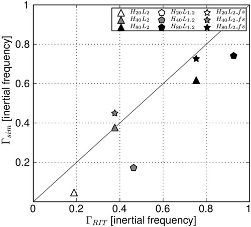
Figure 7. Time-height diagram of the IO horizontal velocity for $H_{20}{L}_2$. The slope of the black line is the vertical phase speed of the IO, $f/m_{IO}$, for the resonant triad involving a $\ast$ wave of frequency $U_G{k}_t-f$ and $m_{IO}>0$. The horizontal white line indicates the height of 1000 m (Colour online).

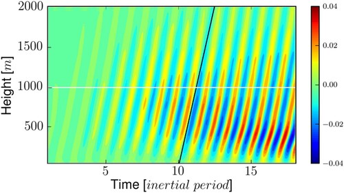
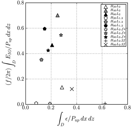
Figure 8. Scatter plot of the IO kinetic energy $E_{IO}$ versus the TKE dissipation rate ϵ integrated over the physical domain D and from 12 to 15 inertial periods. ϵ is scaled by the LW energy flux taken at a height of about 10 m above the topography top and averaged horizontally over the physical domain, denoted $P_{up}$. The IO kinetic energy is scaled by $P_{up}$ during one inertial period $2\pi /f$. Simulations for which the inverse of the IO growth rate is smaller than 3 inertial periods are indicated with a filled marker (black or grey). For simulations with empty markers, the inverse of the IO growth rate is larger than 10 inertial periods. The + and × signs refer to simulations with Coriolis frequency $2f$, for which ${\Gamma }^2<0$.