The inherent instability of axisymmetric magnetostrophic dynamo models

Figures & data

Figure 1. Surface plot of the normalised instantaneous rate of change of magnetic field over the core volume, $I_V$, as a function of the l = 1, n = 1 and l = 1, n = 2 toroidal coefficients β and γ respectively. The vertical black line corresponds to the coefficient values of the known stable steady solution of Li et al. (2018). The α-effect form (4(4) $\alpha ={\alpha }_0\frac{729}{16}{r}^8(1-r^2{)}^2\cos \theta ,$(4) ) is used, with an above critical magnitude of ${\alpha }_0=18$. (a) and (b) show the same 3D plot viewed from a different angle (Colour online).

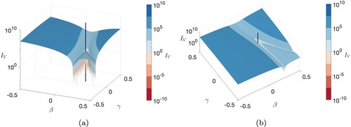
Figure 2. The magnetostrophic trajectory of $I_V$ as a function of toroidal and poloidal energy (defined as half the squared integral over the unit sphere of the respective components). The initial condition is a single poloidal l = n = 1 mode, which is a simple but unsteady Taylor state. The solution evolves from the magenta data point toward a stable steady state with $I_V\ll 1$ and tending to zero. Two magnetic diffusion times of duration are plotted, with circular data points plotted at intervals of 0.001 and blue points denoting when $I_V>1$ and red points when $I_V<1$ (Colour online).

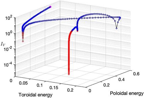
Figure 3. Graphs showing the evolution of (a) $I_V$ and (b) deviation in magnetic energy from the stable state within each symmetry ($\pm {\mathit{B}}_d$ or $\pm {\mathit{B}}_q$ respectively), for the suite of single poloidal mode initial conditions, which fall into either the dipole or quadrupole symmetry class.

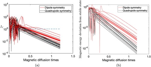
Figure 4. The paths taken from two initial quasi-steady Taylor-state magnetic fields, within (a) dipole symmetry and (b) quadrupole symmetry using the α-effect form (4(4) $\alpha ={\alpha }_0\frac{729}{16}{r}^8(1-r^2{)}^2\cos \theta ,$(4) ) with ${\alpha }_0=18$. The fields diverge from the initial states (magenta points) before finally converging to ${\mathit{B}}_d$ and ${\mathit{B}}_q$ respectively. Blue points denote when $I_V>1$ and red points when $I_V<1$. In (b), the trajectory passes through multiple models which are quasi-steady but unstable. In both cases, convergence to the stable model is denoted by the continuous red line (Colour online).

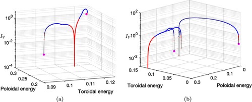
Figure 5. The evolution of four different initial conditions with mixed symmetry (black, blue, red, green) shown by (a) Magnetic energy and (b) $I_V$. The α-effect form (4(4) $\alpha ={\alpha }_0\frac{729}{16}{r}^8(1-r^2{)}^2\cos \theta ,$(4) ) was used with ${\alpha }_0=18$ (Colour online).

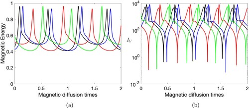
Figure 6. Surface plot of $I_V$ as a function of the l = 1, n = 1 and l = 1, n = 2 toroidal coefficients β and γ respectively. The vertical black line corresponds to the coefficient values of the known stable steady solution of Li et al. (2018). The α-effect form (4(4) $\alpha ={\alpha }_0\frac{729}{16}{r}^8(1-r^2{)}^2\cos \theta ,$(4) ) is used, with an above critical magnitude of ${\alpha }_0=16$. (a) and (b) show the same 3D plot viewed from a different angle.

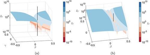
Figure 7. Normalised instantaneous rate of change of magnetic field within the core, $I_V$, with ${\alpha }_0=16$, for 60 different random initial conditions of mixed symmetry.

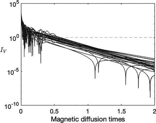
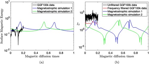
Figure 8. Observational geomagnetic field data from GGF100k (Panovska et al. 2018) are compared to two illustrative models. (a) Total magnetic field core surface energy over the past 100 ka. (b) The instantaneous rate of change of magnetic field at Earth's surface $I_S$ (defined in equation 11(11) $I_V=\frac{\int {\dot{\mathit{B}}}^2\mathrm{d}V}{\int {\mathit{B}}^2\mathrm{d}V},\mathrm{and}{I}_S=\frac{\int {\dot{\mathit{B}}}^2\mathrm{d}S}{\int {\mathit{B}}^2\mathrm{d}S},$(11) ), the GGF100k model, and the resultant field dynamics after passing the data through a Butterworth filter with a 50,000 yr timescale cutoff (red), are compared to the results from the mixed-symmetry simulations of section 4.3 (blue and green). The offset time of GGF100k is arbitrarily chosen to be 0 (Colour online).

Li, K., Jackson, A. and Livermore, P., Taylor state dynamos found by optimal control: axisymmetric examples. J. Fluid Mech. 2018, 853, 647–697.

 Web of Science ®Google Scholar

Panovska, S., Constable, C. and Korte, M., Extending global continuous geomagnetic field reconstructions on timescales beyond human civilization. Geochem. Geophys. Geosyst. 2018, 19, 4757–4772.

 Web of Science ®Google Scholar