
Figures & data
Table 1. Lithuanian benchmark GDP by main sectors of origin in 1937 at current prices.
Figure 1. Map of Lithuania, 1918–1940. Own work, based on Gaučas et al. (Citation2001), Vaskela (Citation2014, pp. 88–89), and calculations in this paper.
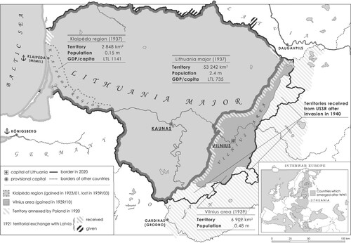
Figure 2. Mean annual population and urbanisation level in Lithuania, 1919–1940. Calculated by the author based on the end-of-the-year population figures, adjusted for dates of territorial changes to arrive at annual mean figures. Urban/rural figures are extrapolated for 1919–1922 and interpolated for 1924–1929 and 1933–1934. Sources: sections on population in Lietuvos statistikos metraštis (Centralinis Statistikos Biuras, Citation1927, Citation1929b, Citation1939a, Citation1940a; Meškauskas, Citation1994, p. 252; Visuotinė Lietuvių Enciklopedija, Citation2016).
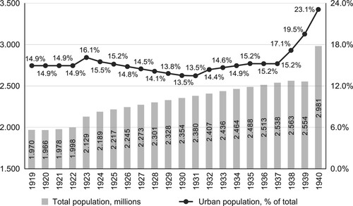
Table 2. Price indices in inter-war Lithuania, 1937 = 100.
Table 3. Volume indices of Lithuanian GVA and its sectors of origin at constant basic prices, 1937 = 100.
Table 4. Total GDP, GDP per capita PPP and cross-checks.
Table 5. Sensitivity analysis.
Figure 3. Lithuanian GDP and GDP per capita at constant prices, 1919–1940. SOURCE: calculations in this paper.
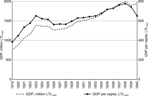
Figure 4. Structure of Lithuanian gross value-added at constant prices, 1919–1940. SOURCE: calculations in this paper.
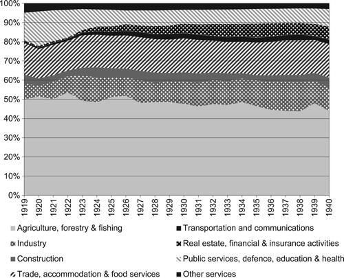
Table 6. Ratio value-added of crops to livestock 1920–1938.
Table 7. Trade (imports plus exports) to GDP ratios in selected countries in 1929 and 1938.
Figure 5. Level of Lithuanian GDP per capita in GK$1990 as percentage of other countries. SOURCE: calculations of this paper, Valge (Citation2003, pp. 2726–2727) and Bolt et al. (Citation2018). The GDP per capita of the post-WW1 emerging states aggregated by dividing the sum of total GDP of those countries by the sum of respective total populations. Western European data taken from Bolt and van Zanden (Citation2014) and includes Austria, Belgium, Denmark, Finland, France, Germany, Italy, Netherlands, Norway, Sweden, Switzerland and the UK.
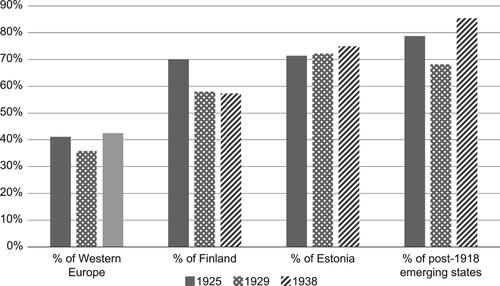
Table 8. Divergence of GDP per capita in post-WW1 emerging states, Group 3 = 100.
Figure 6. Compound annual GDP per capita growth rates in post-WW1 emerging states. Source: calculations of this paper, Valge (Citation2003, pp. 2726–2727), Bolt et al. (Citation2018), Bolt and van Zanden (Citation2020), and Norkus and Markevičiūtė (Citation2021, p. 603).
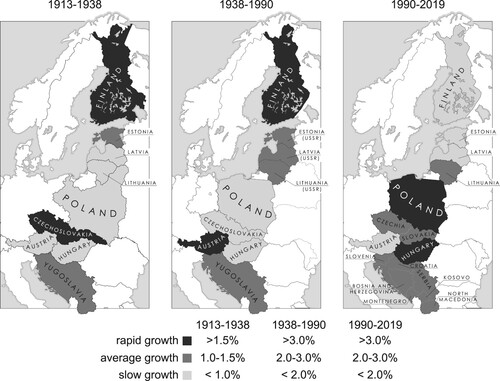
Table A1. Output and value-added of crops, million LTL in 1937 prices.
Table A2. Output and value-added of livestock million LTL in 1937 prices.
Table A3. Value-added of primary sector, million LTL in 1937 prices.
Table A4. Value-added calculations of industry and construction, 1937 = 100 for indices, LTL1937 for monetary values.
Table A5. Value-added of trade, accommodation & food service, transportation and communications, million LTL in 1937 prices.
Table A6. Value-added of FIRE sector, million LTL in 1937 prices.
Table A7. Value-added of public & social security administration, defence, education & health, million LTL in 1937 prices.
Table A8. Value-added of other services, million LTL in 1937 prices.
