A model of ice-marginal sediment-landform development at Lake Tekapo, Southern Alps, New Zealand

Figures & data

Figure 1. (a). Study area location: Mackenzie basin highlighted by dashed box. (b). Mackenzie basin: present-day ice is mapped in white; LGM ice extent is mapped in light grey. (c). 1 m hillshaded bathymetry of Lake Tekapo (from Mountjoy et al. 2019), overlain on a 1 m hillshaded DEM (from Land Information New Zealand; LINZ). The logged outcrop is highlighted by a black box and labelled. The palaeo-lake level at the LGM (Sutherland et al. 2019a, 2019b) is shown by the white contour (726 m a.s.l). Major fault lines are mapped in red (from New Zealand Active Faults Database; NZAFD).

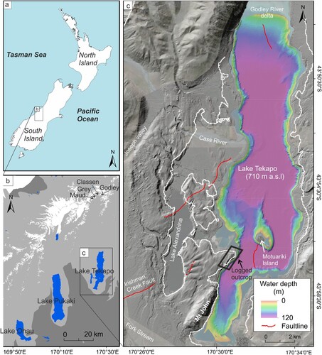
Figure 2. (a). The southwestern shoreline of Lake Tekapo, viewed from the eastern lakeshore, showing the location of the outcrop in panel b and the bedrock contact in panel d. (b). Extent of the logged outcrop, as viewed from the eastern lakeshore. Note that the surface of the cliff is relatively flat-lying, and the top of the outcrop is cut through a palaeo-lake level at 726 m a.s.l. (Sutherland et al. 2019a, 2019b) (c). Contextual photograph to show the vertical scale of the outcrop, viewed from the south. Circle and arrow in the box in panel b indicates the position of the photographer and view direction respectively in panel c. (d). Contact between bedrock and pale silts, location relative to logged exposure shown in panel a.

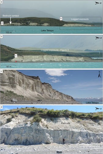
Figure 3. Scaled section sketch of the northern half of the stratigraphic outcrop on the west shoreline of Lake Tekapo, showing main lithofacies and their architectural characteristics. The white area at the base of the section is obscured by talus. Boxed areas are the locations of detailed studies of lithofacies and structures depicted in annotated photographs in Figures 4–12. Readers are directed to the high-resolution online version of this figure for detail.

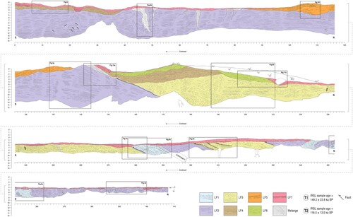
Table 1. Descriptive information and depositional interpretation.

Lithofacies	Facies Code	Brief description	Interpretation	Event/stage
1	Gh (sh)	Horizontally-bedded gravel	Glaciofluvial outwash (bar aggradation)	(i) Ice-margin advance
2	Fl (d)	Laminated rhythmites	Glaciolacustrine varves	(ii) Ice-margin recession
3	St Suc	Cross-bedded sands, coarsening upwards into poorly sorted gravels	Glaciofluvial with hyperconcentrated flow deposits (aggradation in an ice-proximal setting)	(iii) Ice-margin recession
4	Dcs (s) Gms	Interbedded, stratified, and locally clast-supported diamicton and matrix-supported gravels	Sediment gravity flows/hyperconcentrated flows
5	Gfo	Gravel foreset bedding with repetitive grading	Delta foresets	(iv) Advance (Melange horizons developed and glaciotectonic deformation)
6	Dcm	Diamicton	Subglacial mass flow
7	Gms	Poorly-sorted gravels and cross-stratified sands	Glaciofluvial outwash	(a) Ice-margin recession

Facies codes assigned according to Eyles et al. (1983) and Evans and Benn (2004).

Figure 4. Characteristics of LF 1: (a) tilted bedding of well- to poorly-sorted and matrix-supported to clast-supported coarse gravels. Note that gravel packages are separated by discontinuous lenses/beds of laminated silty-sand and silt, displaying soft sediment deformation structures; (b) Stratigraphical and structural interpretation of panel a, location labelled on Figure 3. (c) shear zone/fault contact within LF 1 (outlined and descending from left to right) where upper stratified gravels have been amalgamated with underlying matrix-supported gravels. (d) Clast form for LF 1 collected from area marked by red circle in a.

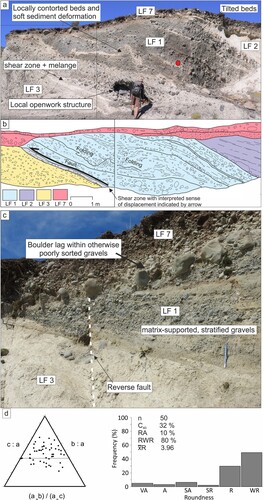
Figure 5. Characteristics of LF 2: (a) coarse and fine grained rhythmite cosets forming repeating couplets and showing strongly developed internal horizontal stratification or lamination (scraper blade = 15 cm long); MS notation = melt season, N-MS notation = non-melt season (b) thin and discontinuous horizontal laminae of coarse sandy silt, displaying rip up clasts and starved ripples, and capped by rapidly fining laminae; (c) lonestone cluster; (d) lonestone (e) rhythmic cycles forming couplets throughout LF 2 and showing the change from thin bedding at the base to the thickest bedding at the top of the sequence. Note the lonestone on the right-hand side of exposure; (f) Stratigraphical and structural interpretation of panel d, location labelled on Figure 3. (g) Heavily faulted and fractured rhythmites (h) Reverse fault with lonestone, note pencil for scale (i) Load and flame soft sediment deformation in sand and silts, note pencil for scale (j) Convoluted and highly contorted sands and silts

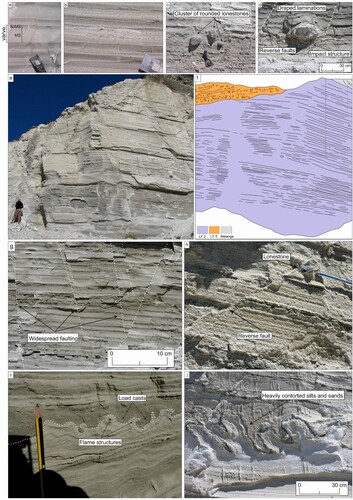
Figure 6. Clastic dykes developed in LF 2: (a) complex of upward-tapering form displaying anabranching gravel-filled necks that isolate blocks of LF 2 host material and end in numerous tapering offshoots and isolated elongate gravel pods or stringers; (b) Stratigraphical and structural interpretation of panel a, location labelled in Figure 3; (c & d) downward-tapering forms, showing also multiple vertical cracks that parallel the wedge sides; (e & f) examples of the bases of downward-tapering wedges, including finer poorly-sorted gravels (d) and finely-laminated rhythmites that parallel the dyke walls (e).

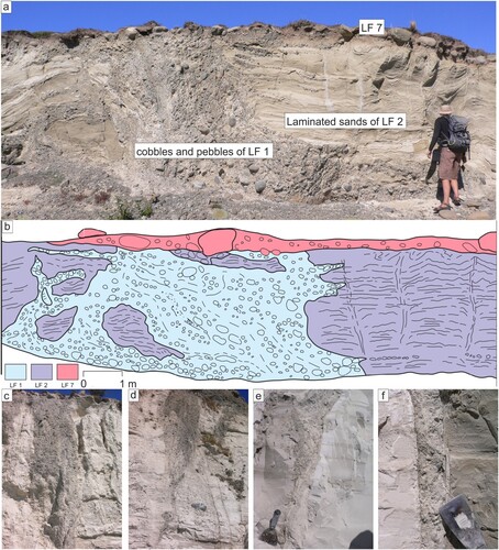
Figure 7. (a) Highly contorted bedding (tight polyclinal folding) displayed in upper LF 2 at the northernmost end of the outcrop. (b) Stratigraphical and structural interpretation of panel a, location labelled in Figure 3 (c) clastic dyke developed along a fault in LF 2, probable hydrofracture (d) close up of probable hydrofracture (e) clastic dyke developed between faults in LF 3

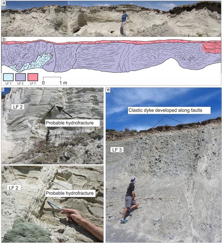
Figure 8. Characteristics of LF 3: (a) packages of massive to crudely horizontally bedded sheets of poorly sorted gravel, separated by discontinuous, lensate bodies of cross-bedded sands; (b) Stratigraphical and structural interpretation of panel a, location labelled on Figure 3; (c) tilted bedding with large concentrations of cross-bedded sands, in thrust fault contact with underlying LF 2 and containing a shallow internal thrust fault dipping northwards; (d) Stratigraphical and structural interpretation of panel c, location labelled on Figure 3; (e) Clast form data from LF 3 sampled from the area marked by the red circle in c.

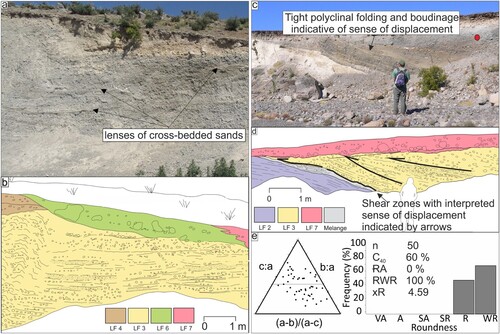
Figure 9. Characteristics of LF 4: (a) outcrop details showing interbedded stratified and locally clast-supported diamictons and matrix-supported gravels, here lying unconformably over LF 2; (b) Stratigraphical and structural interpretation of panel a, location labelled on Figure 3; (c) Clast form data from LF 4.

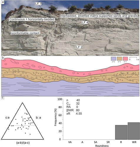
Figure 10. (a) Gravel clinoforms of LF 5 dipping at 20° from right to left and lying unconformably on LF 2 rhythmites and interdigitating vertically with planar bedded gravelly sand and sandy pebble gravel. (b) Stratigraphical and structural interpretation of panel a, location labelled on Figure 3.

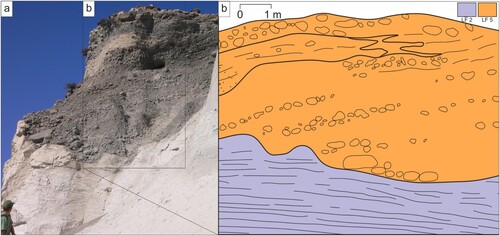
Figure 11. Characteristics of LFs 6 and 7: (a) Stratigraphic overview of LF 6, which is located immediately below the ground surface in this view (indicated above white dashed line) and comprises a massive matrix-supported diamicton (Dmm) overlying LF 3; (b) Nature of the contact between LF 3 and LF 6; (c) Stratigraphical and structural interpretation of panel a, location labelled on Figure 3.

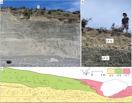
Figure 12. (a) Boulder to cobble gravel of LF 7 and its relationship to LFs 2 and 5; (b) Clast form data from LF 7.

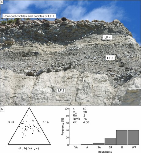
Figure 13. Co-variance graph for RA and C₄₀ value incorporating modern samples from Fox Glacier, collected by Brook and Lukas (2012) and palaeo-data from formerly glaciated sites at the West Coast and Lake Pukaki (Evans et al. 2010, 2013). The C₄₀ values appear unusually slabby compared to other glaciogenic sediments in New Zealand (e.g. Benn and Ballantyne 1994; Evans et al. 2010, 2013a, 2013b; Brook and Lukas, 2012; Lukas et al. 2013). The RWR values also appear elevated and the samples have exceedingly high roundness, indicating very rounded slabs.

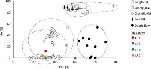
Table 2. Water contents and radionuclide contents.

Field code	Laboratory code	Depth below surface (m)	Water content (%)	^238U (ppm)	^232Th (ppm)	K (%)
T1	WLL1285	15	17.3	2.53 ± 0.02	10.41 ± 0.04	1.31 ± 0.04
T2	WLL1286	0.57	8.7	1.74 ± 0.01	7.14 ± 0.03	1.42 ± 0.01

Figure 14. Conceptual model to illustrate event stratigraphy. (HCF in legend = hyper-concentrated flow, SGF = sediment gravity flow).

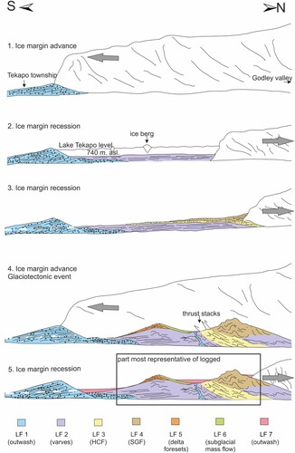
Table 3. Measured a-value and equivalent dose, total dose rate and luminescence age.

Field code	Laboratory code	a-value	Equivalent dose	Calculated cosmic dose rate	Dose rate (Gy/ka)	Luminescence Age (Ka)
T1	WLL1285	0.06 ± 0.02	443.80 ± 9.36	0.0467 ± 0.0023	2.98 ± 0.23	149.2 ± 23.8
T2	WLL1286	0.06 ± 0.02	345.74 ± 2.21	0.2199 ± 0.0110	2.93 ± 0.016	118.0 ± 13.0

Mountjoy JJ, Wang X, Woelz S, Fitzsimons S, Howarth JD, Orpin AR, Power W. 2019. Tsunami hazard from lacustrine mass wasting in Lake Tekapo, New Zealand. Geol Soc. 477(1):413–426.

 Google Scholar

Sutherland JL, Carrivick JL, Shulmeister J, Quincey DJ, James WH. 2019a. Ice-contact proglacial lakes associated with the Last Glacial Maximum across the Southern Alps, New Zealand. Quat Sci Rev. 213:67–92.

 Web of Science ®Google Scholar

Sutherland JL, Carrivick JL, Evans DJA, Shulmeister J, Quincey DJ. 2019b. The Tekapo Glacier, New Zealand, during the Last Glacial Maximum: An active temperate glacier influenced by intermittent surge activity. Geomorphology. 343:183–210.

 Web of Science ®Google Scholar

Eyles N, Eyles CH, Miall AD. 1983. Lithofacies types and vertical profile models; an alternative approach to the description and environmental interpretation of glacial diamict and diamictite sequences. Sedimentology. 30(3):393–410.

 Web of Science ®Google Scholar

Evans DJA, Benn DI. 2004. A practical guide to the study of glacial sediments. London: Hodder Education.

 Google Scholar

Brook MS, Lukas S. 2012. A revised approach to discriminating sediment transport histories in glacigenic sediments in a temperate alpine environment: a case study from Fox Glacier, New Zealand. Earth Surf Processes Landforms. 37(8):895–900.

 Web of Science ®Google Scholar

Evans DJA, Shulmeister J, Hyatt O. 2010. Sedimentology of latero-frontal moraines and fans on the west coast of South Island, New Zealand. Quat Sci Rev. 29(27-28):3790–3811.

 Web of Science ®Google Scholar

Evans DJA, Rother H, Hyatt OM, Shulmeister J. 2013. The glacial sedimentology and geomorphological evolution of an outwash head/moraine-dammed lake, South Island, New Zealand. Sediment Geol. 284:45–75.

 Web of Science ®Google Scholar

Benn DI, Ballantyne CK. 1994. Reconstructing the transport history of glaciogenic sediments – a new approach based on the co-variance of clast form indexes. Sediment Geol. 91(1–4):215–227.

 Web of Science ®Google Scholar

Evans DJA. 2013a. Glacial landsystems. In: Elias SA, Mock C, editors. Encyclopedia of quaternary science. Oxford: Elsevier; p. 813–824.

 Google Scholar

Evans DJA. 2013b. The glacial and periglacial research – geomorphology and retreating glaciers. In: J. Shroder, R. Giardino, J. Harbor, editor. Treatise on geomorphology, vol. 8, glacial and periglacial geomorphology. San Diego, CA: Academic Press; p. 460–478.

 Google Scholar

Lukas S, Benn DI, Boston CM, Brook M, Coray S, Evans DJA, Graf A, Kellerer-Pirklbauer A, Kirkbride MP, Krabbendam M, et al. 2013. Clast shape analysis and clast transport paths in glacial environments: a critical review of methods and the role of lithology. Earth Sci Rev. 121:96–116.

 Web of Science ®Google Scholar