Insights from four decades of model development on the Waterloo Moraine: A review

Figures & data

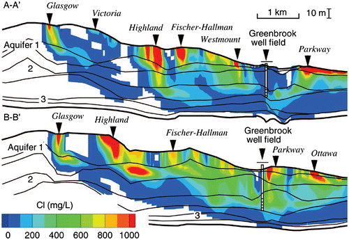
Figure 1. Quasi-three-dimensional multi-aquifer system (from Rudolph and Sudicky 1990, with permission).

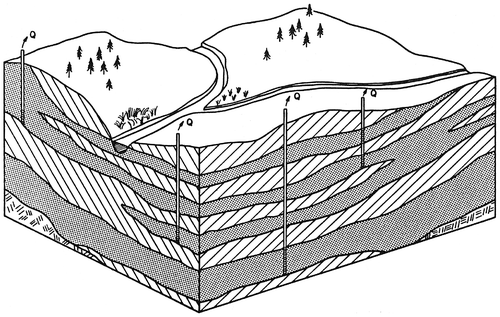
Figure 2. Waterloo Moraine model area (from Martin and Frind 1998, with permission).

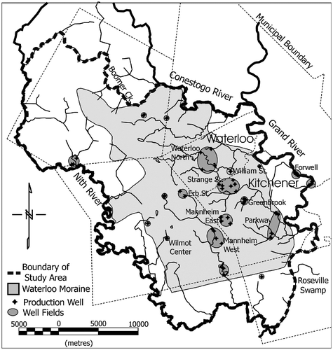
Figure 3. Waterloo Moraine, typical stratigraphic cross-section (from Martin and Frind 1998, with permission). a.s.l., above sea level.

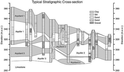
Figure 4. Waterloo Moraine conceptual model (from Martin and Frind 1998, with permission).

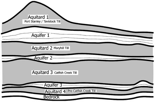
Figure 5. Waterloo Moraine model, three-dimensional finite element grid (from Martin and Frind 1998, with permission).

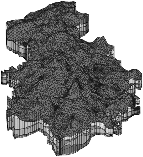
Figure 6. Waterloo Moraine model, simulated hydraulic heads in Aquifer 1 (from Martin and Frind 1998, with permission). mAMSL, meters above mean sea level.

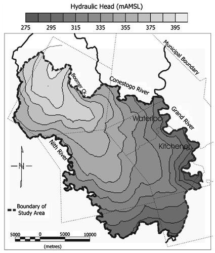
Figure 7. Greenbrook well field, particle tracks in plan view and in cross-section at 280 years (from Frind and Molson 2004).

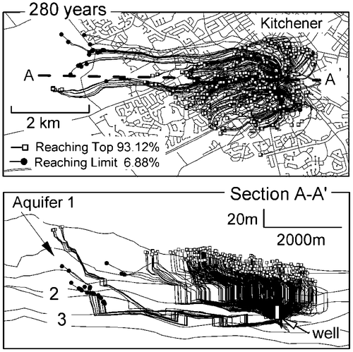
Figure 8. Greenbrook well field, capture probability plumes at 40 and 280 years, maximum value over depth; bottom: cross-section at 40 years (from Frind et al. 2002, with permission).

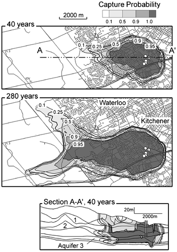
Figure 9. Greenbrook well field: (a) steady-state life expectancy vs. (b) 60-year capture probability (from Molson and Frind 2012).

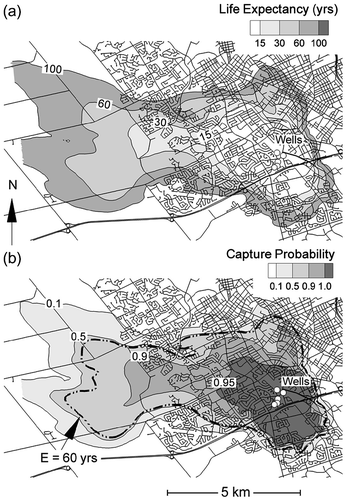
Figure 10. Typical breakthrough curve for well vulnerability mapping (Frind et al. 2006, with permission).

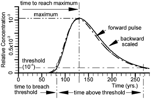
Figure 11. Well vulnerability maps for Mannheim well: (a) maximum relative concentration; (b) time taken (from Rahman et al. 2010).

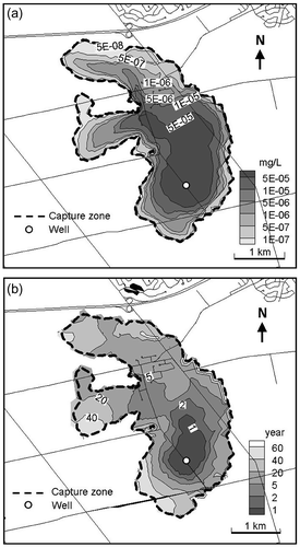
Figure 12. Capture probability maps for Mannheim well: (a) single-scenario analysis (WATFLOW), protection objective; (b) multi-scenario analysis, protection objective; (c) multi-scenario analysis, mitigation objective (from Sousa et al. 2013). The 0.5 contour has been emphasized.

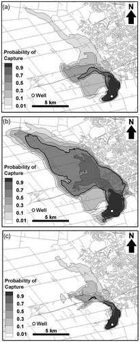
Figure 13. Greenbrook well field, chloride distributions in plan view at (a) ground surface, (b) detailed view at ground surface and (c) in pumped aquifer (from Bester et al. 2006, with permission).

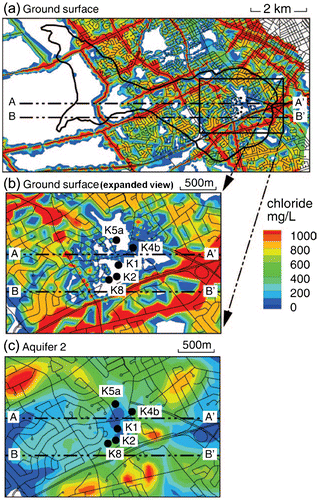
Figure 14. Greenbrook well field, chloride distributions, cross-sectional view (from Bester et al. 2006, with permission). Arterial roads indicated. Cl, chloride.

Rudolph, D. L., and E. A. Sudicky. 1990. Simulation of groundwater flow in complex multiaquifer systems: Performance of quasi three-dimensional technique in the steady-state case. Canadian Geotechnical Journal 27: 590–600.

 Web of Science ®Google Scholar

Martin, P. J., and E. O. Frind. 1998. Modeling a complex multi-aquifer system: The Waterloo Moraine. Ground Water 36(4): 679–690.

 Web of Science ®Google Scholar

Frind, E. O., and J. W. Molson. 2004. A new particle tracking algorithm for finite element grids. Keynote lecture presented at Finite-Element Models, MODFLOW, and More Conference (sponsored by Int. Assoc. of Hydrological Sciences and US Geological Survey), Carlsbad, Czechia, 13–16 Sept. 2004.

 Google Scholar

Frind, E. O., D. S. Muhammad, and J. W. Molson. 2002. Delineation of three-dimensional capture zones in complex multi-aquifer systems. Ground Water 40(6): 586–589.

 PubMed Web of Science ®Google Scholar

Molson, J. W., and E. O. Frind. 2012. On the use of mean groundwater age, life expectancy and capture probability for defining aquifer vulnerability and time-of-travel zones for source water protection. Journal of Contaminant Hydrology 127: 76–87.

 PubMed Web of Science ®Google Scholar

Rahman, R., E. O. Frind, and D. L. Rudolph. 2010. Assessing the impact of Beneficial Management Practices for controlling nitrate concentrations in well water. In Proceedings, GQ10, Groundwater Quality Management in a rapidly changing world, 7th International Groundwater Quality Conference, Zurich, Switzerland, 13–18 June. Editors M. Schirmer, E. Hoehn and T. Vogt. IAHS Publ. 342, 2011, 326–329. Wallingford, UK: IAH Press.

 Google Scholar

Sousa, M. R., E. O. Frind, and D. L. Rudolph. 2013. An integrated approach for addressing uncertainty in the delineation of groundwater management areas. Journal of Contaminant Hydrology 148: 12–24.

 PubMed Web of Science ®Google Scholar

Bester, M., E. O. Frind, J. W. Molson, and D. L. Rudolph. 2006. Numerical investigation of road salt impact on an urban well field. Ground Water 44(2): 165–175.

 PubMed Web of Science ®Google Scholar