875
Views
9
CrossRef citations to date
0
Altmetric
Articles

Variability of tracer breakthrough curves in mountain streams: Implications for streamflow measurement by slug injection

, &
Pages 21-37 | Received 19 Feb 2016, Accepted 11 Jul 2016, Published online: 22 Aug 2016

Figures & data

Table 1. Salt dilution dosage guidelines from various sources.

Table 2. Characteristics of stream reaches used in the study.

Figure 1. Locations of study stream sites (black circles) in British Columbia. Sites are identified as follows: BG – Bridge Glacier watershed (Bridge Glacier West Creek and Bridge Glacier South Creek); Pl – Place Creek; Cy – Cayoosh Creek, Pe – Pemberton Creek; R – Rutherford Creek; M – Mosquito Creek; CC – Carnation Creek watershed (Carnation Creek Tributary C and Carnation Creek Tributary L).
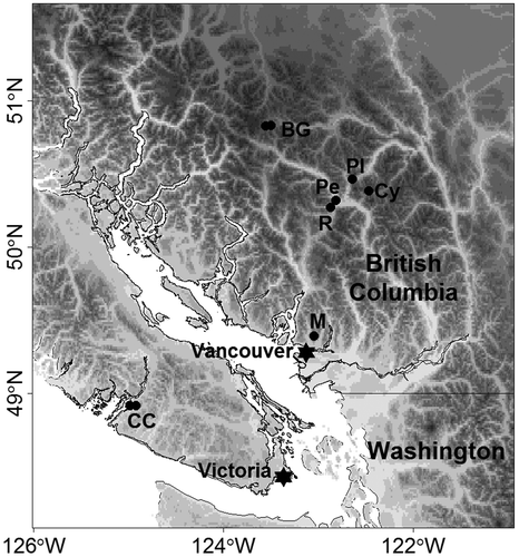
Figure 1. Locations of study stream sites (black circles) in British Columbia. Sites are identified as follows: BG – Bridge Glacier watershed (Bridge Glacier West Creek and Bridge Glacier South Creek); Pl – Place Creek; Cy – Cayoosh Creek, Pe – Pemberton Creek; R – Rutherford Creek; M – Mosquito Creek; CC – Carnation Creek watershed (Carnation Creek Tributary C and Carnation Creek Tributary L).

Figure 2. Examples of experimental setups at (a, b, c) Rutherford Creek and (d) Pemberton Creek. For reference for Rutherford Creek, the distance from the injection point to the location where complete mixing was verified was 140 m and the mean wetted width was 7.7 m. For reference for Pemberton Creek, the mean wetted width was 10.0 m.
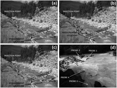
Figure 2. Examples of experimental setups at (a, b, c) Rutherford Creek and (d) Pemberton Creek. For reference for Rutherford Creek, the distance from the injection point to the location where complete mixing was verified was 140 m and the mean wetted width was 7.7 m. For reference for Pemberton Creek, the mean wetted width was 10.0 m.

Table 3. Mixing lengths determined from discharge measurements at multiple locations. “Mixing length assumed from same-side probes” indicates that two measurement probes on the same side of the stream measured similar discharges, while “mixing length assumed from opposite-side probes” indicates that two measurement probes on opposite sides of the stream measured similar discharges. “NA” indicates that there were probes on only one side of the stream. Note that some streams have different mixing lengths based on discharge.

Table 4. Discharge measurements (m3·s−1) for Carnation Creek Trib C. Reach length (m) for each probe is in parentheses. From visual field observation, the wetted width was between 1.5 m and 2.0 m for Injections 1 through 5, and unknown for Injection 6.

Figure 3. Breakthrough curves (BTCs) for discharge measurements focused on measurement location variability. One sample injection for each stream. Different plotting symbols are the BTCs for different probes for the same injection: (a) Carnation Creek Trib C Injection 3 (Q = 0.040 m3·s−1 ± 4.4%; (b) Carnation Creek Trib L Injection 2 (Q = 0.0090 m3·s−1 ± 4.3%; (c) Mosquito Creek Injection 1 (Q = 0.349 m3·s−1 ± 2.9%; (d) Pemberton Creek Injection 5 (Q = 2.14 m3·s−1 ± 2.7%. EC – electrical conductivity.
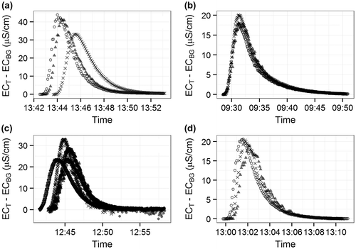
Figure 3. Breakthrough curves (BTCs) for discharge measurements focused on measurement location variability. One sample injection for each stream. Different plotting symbols are the BTCs for different probes for the same injection: (a) Carnation Creek Trib C Injection 3 (Q = 0.040 m3·s−1 ± 4.4%; (b) Carnation Creek Trib L Injection 2 (Q = 0.0090 m3·s−1 ± 4.3%; (c) Mosquito Creek Injection 1 (Q = 0.349 m3·s−1 ± 2.9%; (d) Pemberton Creek Injection 5 (Q = 2.14 m3·s−1 ± 2.7%. EC – electrical conductivity.

Table 5. Discharge measurements for injections focusing on measurement location variability. The value of is a measure of the percent error in measured discharge for one injection.

Figure 4. Plots of all non-dimensional breakthrough curves (BTCs): (a) BTCs with A* values between 0.24 and 0.49 (n = 51), (b) BTCs with A* values between 0.49 and 0.62 (n = 67), and (c) BTCs with A* values between 0.62 and 0.94 (n = 51).
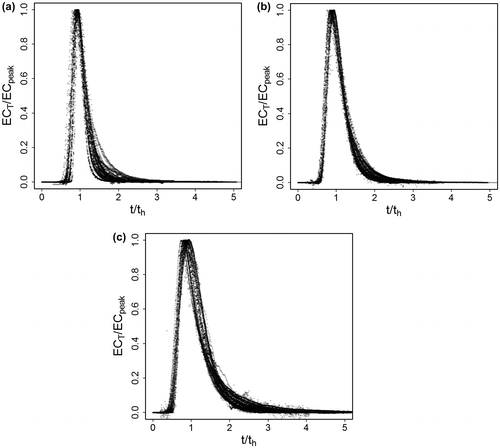
Figure 4. Plots of all non-dimensional breakthrough curves (BTCs): (a) BTCs with A* values between 0.24 and 0.49 (n = 51), (b) BTCs with A* values between 0.49 and 0.62 (n = 67), and (c) BTCs with A* values between 0.62 and 0.94 (n = 51).

Figure 5. Boxplot of A* values for all injections from all streams (field study streams and Northwest Hydraulic Consultants Ltd. streams). EC – electrical conductivity.
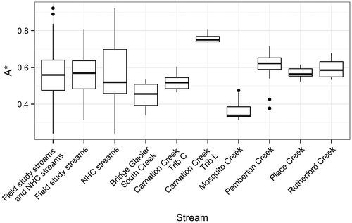
Figure 5. Boxplot of A* values for all injections from all streams (field study streams and Northwest Hydraulic Consultants Ltd. streams). EC – electrical conductivity.

Figure 6. Histograms of A* values: (a) Field study streams (n = 121); (b) Northwest Hydraulic Consultants Ltd. (NHC) streams (n = 54).
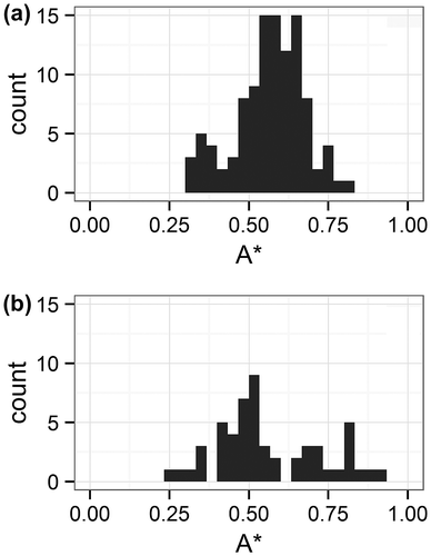
Figure 6. Histograms of A* values: (a) Field study streams (n = 121); (b) Northwest Hydraulic Consultants Ltd. (NHC) streams (n = 54).

Figure 7. Variability of A* with discharge, for all injections from all field study streams (n = 121). The black line is a linear regression fit to provide visual reference (p < 0.001, adjusted R2 = 0.16).
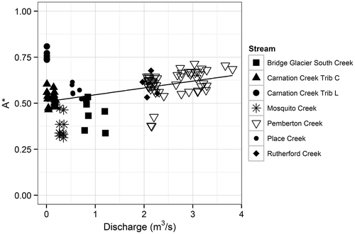
Figure 7. Variability of A* with discharge, for all injections from all field study streams (n = 121). The black line is a linear regression fit to provide visual reference (p < 0.001, adjusted R2 = 0.16).

Figure 8. Variability of A* with ratio of reach length to wetted width, for all injections from all field study streams (n = 121). The black line is a linear regression fit to provide visual reference (p < 0.001, adjusted R2 = 0.30).
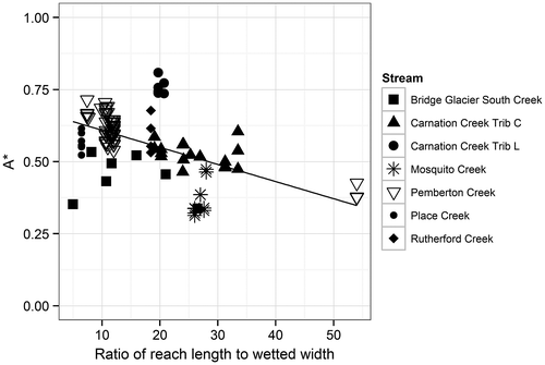
Figure 8. Variability of A* with ratio of reach length to wetted width, for all injections from all field study streams (n = 121). The black line is a linear regression fit to provide visual reference (p < 0.001, adjusted R2 = 0.30).

Figure 9. Variability of A* with discharge, for a constant reach length, at Pemberton Creek. The relation was weak and not quite significant (p = 0.053).
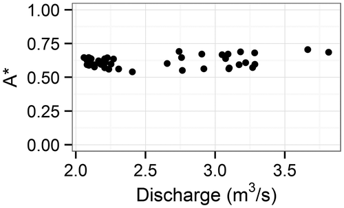
Figure 9. Variability of A* with discharge, for a constant reach length, at Pemberton Creek. The relation was weak and not quite significant (p = 0.053).

Figure 10. Variability of A* with reach length, for constant discharge, at Carnation Creek Trib C. The black line is linear regression relation for all injections (p < 0.001).
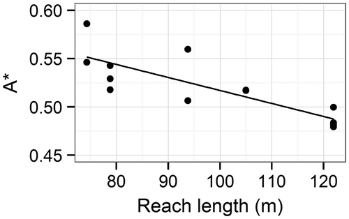
Figure 10. Variability of A* with reach length, for constant discharge, at Carnation Creek Trib C. The black line is linear regression relation for all injections (p < 0.001).

Table 6. Measurement location variability of A*. Highest/lowest A* is the highest/lowest average A* value from one probe for all injections at that stream. In the location description, the value in brackets is a visual estimate of the ratio of the local velocity near the probe to the maximum local velocity across the channel.

Table 7. Example salt dosage calculation using A* and Equation (11).

Reprints and Corporate Permissions

Please note: Selecting permissions does not provide access to the full text of the article, please see our help page How do I view content?

To request a reprint or corporate permissions for this article, please click on the relevant link below:

Academic Permissions

Please note: Selecting permissions does not provide access to the full text of the article, please see our help page How do I view content?

Obtain permissions instantly via Rightslink by clicking on the button below:

If you are unable to obtain permissions via Rightslink, please complete and submit this Permissions form. For more information, please visit our Permissions help page.