Figures & data
Figure 1. (A) Study area in Saskatchewan, Canada, shown with false color (Red: shortwave infrared band, Green: infrared band, Blue: red band) Landsat best-available-pixel (BAP) composite relating 2015 conditions overlaid with forested ecozones. Inset map displays its location in Canada. (B) Spatial distribution of burned forests in 1985 to 1994 and 1995 to 2014 (the latter period was used to build the burn probability model) detected from Landsat time-series data in relation to unburned forests over the 1985 to 2014 period. (C) Topography of the study area. (For interpretation of the references to color in this figure legend, the reader is referred to the online version of this article.)
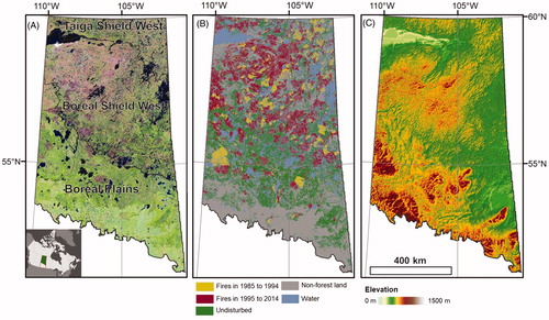
Figure 2. Workflow for integrating Landsat and ancillary data for modeling burn probability.
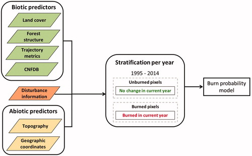
Table 1. Predictor variables used to model burn probability.
Figure 3. Variable importance for the burn probability Random Forests model.
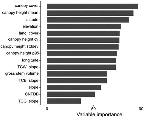
Table 2 Confusion matrix of the estimated proportions of area for the burn probability prediction model for calibration data 1995–2014.
Figure 4. Partial dependence plots for biotic variables on burn probability: (A) canopy height mean and canopy height standard deviation, (B) canopy cover and gross stem volume. The inner ticks along the x-axes represent deciles of the predictor variables.
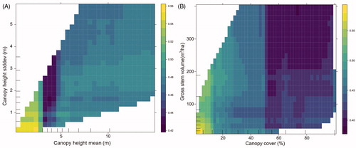
Figure 5. Partial dependence plots for (A) land cover and (B) temporal trajectory metrics on burn probability, depicting the relationship between burn probability and long-term spectral trends. The inner ticks along the x-axes represent deciles of the predictor variables.
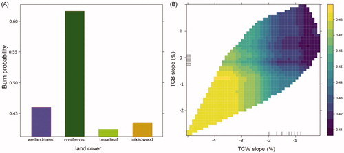
Figure 6. Partial dependence plots for (A) geographic and (B) topographic controls on burn probability. The inner ticks along the x-axes represent deciles of the predictor variables.
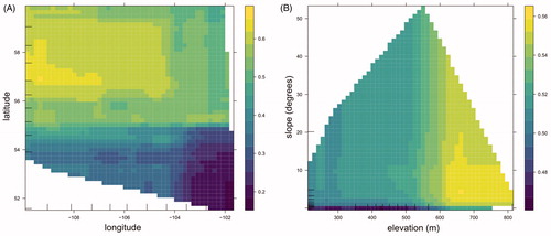
Figure 7. (A) Predicted forest burn probability in 2015 in Saskatchewan’s forested ecosystems, in comparison to actual burned forest areas for 2015, as detected independently by the C2C approach. Zoom-in examples showing spatially detailed agreement between predicted burn probability and detected fires in (B) Boreal Shield West and (C) Boreal Plains.
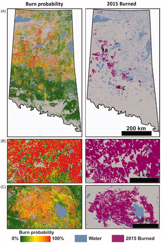
Figure 8. Distribution of predicted burn probability values for burned and unburned treed areas in our study area detected from Landsat time series data. Vertical solid lines represent the median probability for the burned and unburned class. The vertical dotted line represents the median probability for the entire study area.
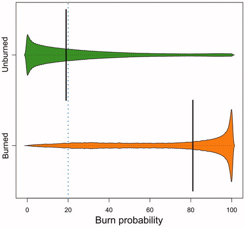
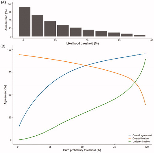
Figure 9. (A) Predicted burned area, and (B) predictive agreement with actual fires in 2015 as function of the threshold applied to burn probability to predict burned areas.