
Figures & data
Figure 1. Political map (panel (a)) and Madre de Dios study area with a Landsat 8 OLI background image in RGB combination: SWIR2, SWIR1 and GREEN bands (panel (b)). Panel (d) shows the Digital Elevation Model (DEM) of the Shuttle Radar Topographic Mission (SRTM), both panel (b) and panel (d) represent the same study area. Panel (c) shows gold mining through PlanetLabs images (at 5 m); in addition, the resolution of this image makes it possible to see the characteristics of the gold mining in the study region (i.e., presence of water bodies).
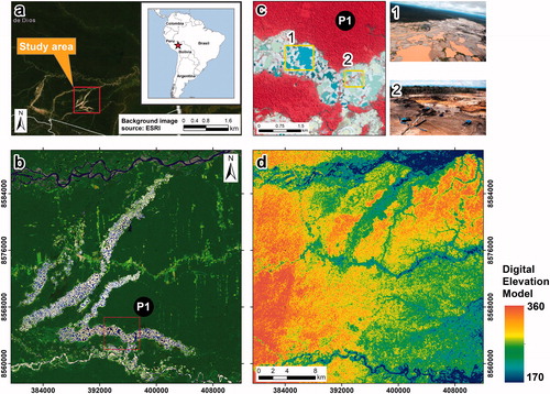
Figure 2. Flowchart of the pre-processing and processing of the optical and SAR images is shown.
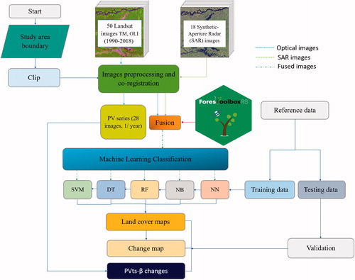
Table 1. Number of tie points, threshold of accuracy and RMSE in pixel units obtained after co-registration between optical and radar data.
Figure 3. Examples of time series of forests that have been deforested (points in blue). The Landsat images in the top row are in combination SWIR2, NIR and RED. The middle row contains the PV fractions scaled between 0 and 100. Finally, the lower row shows the detections made by the PVts-β approach with β = 5. The PV series were smoothed, before detecting deforestation, with the “smootH” function (see Appendix B).
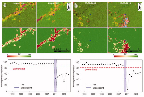
Table 2. Number of points for the calibration of the classifiers and also for obtaining the change cartography for the years 2009 and 2018, as well as samples for validating the changes obtained with the classifiers and the PVts-β approach.
Figure 4. Panel (a) and (b) show the combinations NIR, RED and GREEN and SWIR2, SWIR1, GREEN from the year 2009 (Landsat-5 TM). Panel (c) and (d) show the same region with polarizations HH and HV (ALOS PALSAR—2009) respectively. Panel (e) and (f) show the combinations NIR, RED and GREEN and SWIR2, SWIR1, GREEN from the year 2018 (Landsat-8 OLI). Panel (g) and (h) show the same region with polarizations VV and VH (Sentinel 1B—2018). Finally, panel (i) and (j) show the fused images of 2009 and 2018 respectively, in both cases using a combination with the first three principal components.
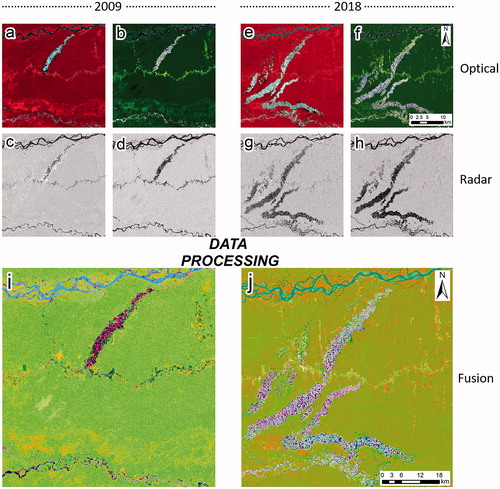
Figure 5. Proportion of variance of each PC and the cumulative variance for the year 2009 is shown in panel (a); panel (b) shows the same for the year 2018.
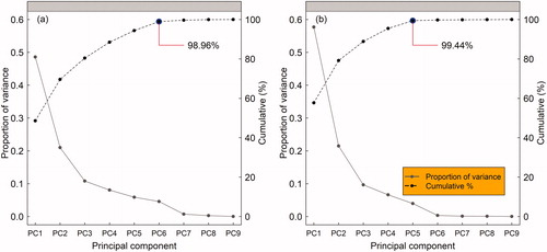
Table 3. Contribution in percentages (%) of the variables to the principal components after the fusion of optical and SAR images for the years 2009 and 2018.
Figure 6. The calibrations were performed through CV and MCCV, panel (a) is for the year 2009 and panel (b) is for the year 2018. The minimum, maximum and average of the overall accuracies for each algorithm are shown. In addition, we show the variance obtained for the k = 10 groups and for 100 iterations.
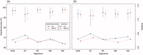
Figure 7. Classifications using the six principal components of the fused image in the year 2009. Panels (a), (b), (c)*, (d) and (e) represent the classifications obtained with SVM, DT, RF (*the highest overall accuracy), NB and NN, respectively.
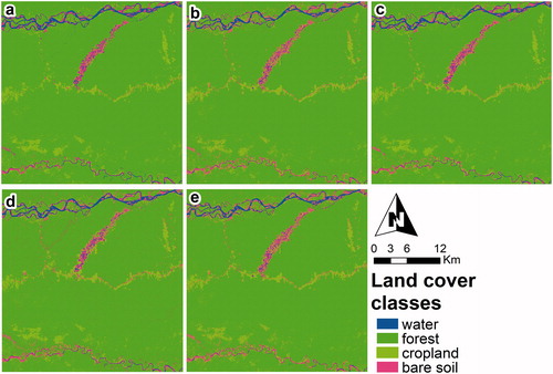
Figure 8. Classifications using the five principal components of the fused image in the year 2018. Panels (a), (b), (c), (d) and (e)* represent the classifications obtained with SVM, DT, RF, NB, and NN (*the highest overall accuracy) respectively. Class “Difference*” represents the difference map of the same classifier between 2009 and 2018 with ground truth (Hansen et al. Citation2013).
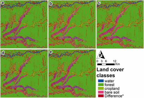
Table 4. Overall accuracy and Kappa index for all classification algorithms and both dates.
Figure 9. Panel (a) and (b) show deforestation detections (2009–2018) obtained from the PVts-β approach and the RF-NN classifiers respectively. Panel (c) and (d) show the reference data from Hansen et al. (Citation2013) and MINAM respectively. All the panels have the SWIR1, NIR and RED combination from the year 2018 (Landsat 8 OLI) as the background.
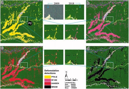
Table 5. Overall accuracy, kappa index, and the average commission and omission errors (average commissions and omissions from deforestation classes and intact forest) are shown for the PVts-β approach, and for the change obtained with the RF-NN classifiers.
Figure 10. Column (a) shows SAR images without a speckle filter, column (b) images with SSF, column (c) shows a Multi-temporal Speckle Filter (MSF). To evaluate the reduction of speckle noise we used three indicators: (i) visual interpretation, (ii) Signal Level Ratio (SLR) (White et al. Citation2020), and (iii) the standard deviation of the intensity before and after applying filters for areas with higher signal echo intensity (P3) and areas with lower signal echo intensity (P4) (column d). The parameters for the MSF filter were used by default: (i) filter: filter Lee, (ii) Number of looks: 1, (iii) Window size: 7 × 7, and (iv) Sigma: 0.9.
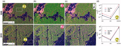
Table 6. SLR is a ratio of the unfiltered image to the filtered image averaged over a region (R1 and R2).