Water Bottom and Surface Classification Algorithm for Bathymetric LiDAR Point Clouds of Very Shallow Waters

Figures & data

Table 1. Summary of the bathymetric LiDAR classification methods.

Study	Analysis		Classified objects		Methods		Sensor
	Full waveform	Point cloud	Water bottom	Water surface	Parametric approach	Machine learning
Xing et al. 2019	✓	–	✓	✓	✓	–	Mapper5000
Schwarz et al. 2019	✓	–	✓	✓	✓	–	Riegl VQ-880-G
Mader et al. 2019	✓	–	✓	–	✓	–	Riegl VQ-880-G
Ma et al. 2019	✓	–	✓	✓	✓	–	Optech Aquarius
Yang et al. 2022	✓	–	✓	✓	✓	–	Mapper5000
Kogut et al. 2022	–	✓	✓	✓	–	✓	Leica AHAB Chiroptera I
Kogut and Weistock 2019	–	✓	✓	✓	–	✓	Leica AHAB Chiroptera I
Lowell and Calder 2021a	–	✓	✓	–	–	✓	Riegl VQ-880-G
Lowell and Calder 2021b	–	✓	✓	–	✓	✓	Riegl VQ-880-G
Mandlburger et al. 2015	✓	✓	✓	✓	✓	–	Riegl VQ-820-G & VQ-880-G
Yang et al. 2020	–	✓	✓	–	✓	–	Optech Aquarius
Jung et al. 2021	–	✓	✓	–	✓	–	Riegl VQ-880-G

Figure 1. Test site: (a) Marco Island in Florida, USA and VQ-880-G point cloud data and (b) Samcheok in Gangwon-Do, South Korea and Seahawk point cloud data.

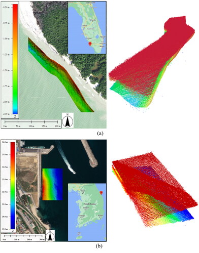
Table 2. Summary of the test datasets.

System	Location	Year	Area (m^2)	Number of points	Point density (pts/m^2)	Z range (m)	Water depth range (m)
Riegl VQ-880-G	Marco Island, Florida, USA	2016	14,192	697,044	49.12	−13.30 ∼ −0.09	0 ∼ 1.81
Seahwak	Donghae, Gangwon-Do, South Korea	2022	40,320	129,125	3.20	18.60 ∼ −26.27	0.30 ∼ 7.28

Figure 2. Examples of (a) waveform decomposition; (b) water levels; and (c) pseudo-waveform decomposition.

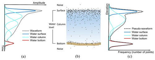
Figure 3. Key steps of the proposed workflow: (a) 2D grid cell structure generation; (b) point cloud that falls onto a single cell; (c) pseudo-waveform generation; (d) pseudo-waveform decomposition; (e) pseudo-waveform classification; and (f) classified point cloud.

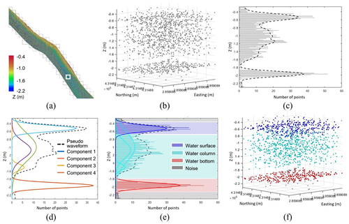
Figure 4. Workflow of the pseudo-waveform decomposition.

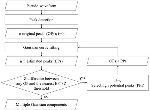
Figure 5. Iterative Gaussian decomposition of pseudo-waveform by estimating the potential peaks: (a) original peak detection; (b,c) estimation of the potential peak through Gaussian curve fitting; (d) pseudo-waveform decomposition result.

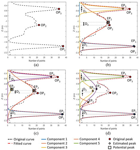
Figure 6. Examples of the classification bound determination with (a) four components; (b) two separate components; (c) two intersecting components.

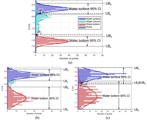
Table 3. Test variables for sensitivity analysis.

Parameter	Unit	Test variables
Cell size (χ)	Meters	5, 10, 15, 20, 25
Smoothing filter size (σ)	Unitless	1, 2, 3, 4
Z threshold (τ)	Meters	0.1, 0.2, 0.3, 0.4, 0.5

Table 4. Top 10 combinations of parameters in descending order of overall accuracy for VQ-880G data.

Rank	Parameters						Accuracy				Efficiency (1000 points/s)
	Cell size (m)	Filter size	Z threshold (m)	Water bottom			Water surface			Overall accuracy (%)
				Precision (%)	Recall (%)	F1 score (%)	Precision (%)	Recall (%)	F1 score (%)
1	5	2	0.3	99.240	98.649	98.944	81.738	98.715	89.428	91.234	39.815
2	5	2	0.5	99.241	98.649	98.944	81.720	98.716	89.417	91.225	41.963
3	5	2	0.4	99.241	98.649	98.944	81.719	98.716	89.416	91.224	43.707
4	5	2	0.2	99.225	98.345	98.783	81.680	98.603	89.348	91.052	26.877
5	5	2	0.1	99.227	98.214	98.718	81.587	98.506	89.252	90.928	20.215
6	5	1	0.5	99.520	87.899	93.349	85.087	95.908	90.174	88.014	4.450
7	5	1	0.3	99.520	87.907	93.354	85.189	95.727	90.151	88.012	3.837
8	5	1	0.4	99.520	87.899	93.349	85.069	95.899	90.160	88.004	4.459
9	10	2	0.5	98.211	89.259	93.521	82.929	98.381	89.997	87.839	34.762
10	10	2	0.4	98.211	89.259	93.521	82.913	98.381	89.987	87.831	23.614

Table 5. Bottom 10 combinations of parameters in ascending order of overall accuracy for VQ-880G data.

Rank	Parameters						Accuracy				Efficiency (1000 points/s)
	Cell size (m)	Filter size	Z threshold (m)	Water bottom			Water surface			Overall accuracy (%)
				Precision (%)	Recall (%)	F1 score (%)	Precision (%)	Recall (%)	F1 score (%)
1	20	1	0.1	99.070	21.005	34.661	85.744	95.518	90.367	62.747	2.590
2	20	1	0.2	99.057	22.227	36.307	85.395	97.473	91.035	63.641	4.213
3	20	1	0.3	99.254	23.869	38.484	85.202	97.480	90.929	64.211	11.540
4	20	1	0.4	99.182	23.894	38.511	85.296	97.464	90.975	64.260	17.591
5	20	1	0.5	99.183	23.925	38.550	85.310	97.457	90.980	64.279	19.814
6	25	1	0.5	97.324	25.964	40.992	84.903	97.925	90.950	64.799	16.711
7	25	1	0.4	97.324	25.964	40.992	84.942	97.925	90.972	64.818	16.081
8	25	1	0.1	99.179	25.327	40.349	85.624	97.696	91.263	64.938	3.917
9	25	1	0.2	98.837	26.419	41.693	85.305	97.754	91.106	65.190	6.243
10	25	1	0.3	97.678	29.613	45.448	85.180	97.849	91.076	66.299	12.567

Figure 7. Sensitivity analysis that accounts for both water bottom and surface with respect to three parameters: (a) cell size; (b) smoothing filter size; (c) Z threshold.

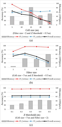
Table 6. Performance comparison of the water bottom classification methods for VQ-880G data.

Method	Precision (%)	Recall (%)	F1 score (%)
Provided	99.896	90.562	95.000
k-means	92.024	98.522	95.162
Inverse histogram	97.360	97.390	97.375
Proposed	99.240	98.649	98.944

Figure 8. Classified water bottom points of VQ-880G data: (a–e) close-up view of region #1; and (f–j) close-up view of region #2.

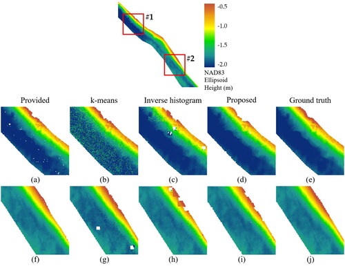
Figure 9. Examples of classification results by depth and water bottom type: (a) clear separation of the water bottom (depth < 1.7 m); (b,c) unclear separation of the water bottom (depth < 1.3 m); (d) very shallow water (depth < 0.7 m); (e) uneven water bottom (depth < 1 m).

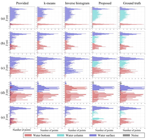
Table 7. Optimized parameters and accuracies of the classification result of Seahawk data.

Parameters			Accuracy (%)
Cell size	Filter size	Z threshold	Water bottom			Water surface			Overall accuracy
			Precision	Recall	F1 score	Precision	Recall	F1 score
20 m	4	0.3 m	99.378	98.272	98.822	99.031	97.788	98.406	97.291

Figure 10. Error distribution in the Z-direction (ΔZ) of Seahawk data: (a) classified water bottom points; (b) MBES data; (c) the difference map of ΔZ; (d) frequency histogram of ΔZ.

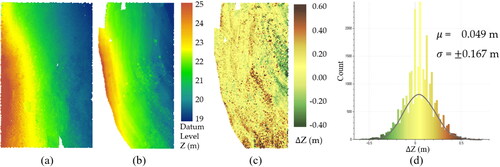
Table A1. Specifications for Riegl VQ-880G system.

Parameter	Specification
Laser wavelength	532 nm (green) 1064 nm (NIR)
Laser pulse width	1.6 ns
Laser beam divergence	0.7–2.0 mrad (green) 0.2 mrad (NIR)
Field of view (FoV)	40°
Pulse repetition rate	550 kHz
Operating flight altitude	600 m
Minimum range (1.5 Secchi depth)	10 m
Main dimensions (L × W × H)	444 × 444 × 695 mm
Weight	65 kg

Table A2. Specifications for Seahawk system.

Parameter	Specification
Laser wavelength	532 nm (green) 1064 nm (NIR)
Laser pulse width	1.7 ns
Laser beam divergence	7 mrad (green) 10.5 mrad (NIR)
Field of view (FoV)	20°
Pulse repetition rate	10 kHz
Operating flight altitude	400 m
Minimum range (1.5 Secchi depth)	10 m
Main dimensions (L × W × H)	442 × 515 × 499 mm
Weight	73 kg

Xing, S., Wang, D., Xu, Q., Lin, Y., Li, P., Jiao, L., Zhang, X., and Liu, C. 2019. “A depth-adaptive waveform decomposition method for airborne LiDAR bathymetry.” Sensors, Vol. 19(No. 23): pp. 5065. doi:10.3390/s19235065.

 PubMed Web of Science ®Google Scholar

Schwarz, R., Mandlburger, G., Pfennigbauer, M., and Pfeifer, N. 2019. “Design and evaluation of a full-wave surface and bottom-detection algorithm for LiDAR bathymetry of very shallow waters.” ISPRS journal of Photogrammetry and Remote Sensing, Vol. 150: pp. 1–10. doi:10.1016/j.isprsjprs.2019.02.002.

 Web of Science ®Google Scholar

Mader, D., Richter, K., Westfeld, P., Weiß, R., and Maas, H.G. 2019. “Detection and extraction of water bottom topography from laser bathymetry data by using full-waveform-stacking techniques.” The International Archives of the Photogrammetry, Remote Sensing and Spatial Information Sciences, Vol. XLII-2/W13: pp. 1053–1059. doi:10.5194/isprs-archives-XLII-2-W13-1053-2019.

 Google Scholar

Ma, Y., Zhang, J., Zhang, Z., and Zhang, J.Y. 2019. “Bathymetry retrieval method of LiDAR waveform based on multi-Gaussian functions.” Journal of Coastal Research, Vol. 90(No. sp1): pp. 324–331. doi:10.2112/SI90-041.1.

 Google Scholar

Yang, F., Qi, C., Su, D., Ding, S., He, Y., and Ma, Y. 2022. “An airborne LiDAR bathymetric waveform decomposition method in very shallow water: A case study around Yuanzhi Island in the South China Sea.” International Journal of Applied Earth Observation and Geoinformation, Vol. 109: pp. 102788. doi:10.1016/j.jag.2022.102788.

 Web of Science ®Google Scholar

Kogut, T., Tomczak, A., Słowik, A., and Oberski, T. 2022. “Seabed Modelling by Means of Airborne Laser Bathymetry Data and Imbalanced Learning for Offshore Mapping.” Sensors, Vol. 22(No. 9): pp. 3121. doi:10.3390/s22093121.

 PubMed Web of Science ®Google Scholar

Kogut, T., and Weistock, M. 2019. “Classifying airborne bathymetry data using the Random Forest algorithm.” Remote Sensing Letters, Vol. 10(No. 9): pp. 874–882. doi:10.1080/2150704X.2019.1629710.

 Web of Science ®Google Scholar

Lowell, K., and Calder, B. 2021a. “Assessing marginal shallow-water bathymetric information content of lidar sounding attribute data and derived seafloor geomorphometry.” Remote Sensing, Vol. 13(No. 9): pp. 1604. doi:10.3390/rs13091604.

 Web of Science ®Google Scholar

Lowell, K., and Calder, B. 2021b. “Extracting shallow-water bathymetry from lidar point clouds using pulse attribute data: merging density-based and machine learning approaches.” Marine Geodesy, Vol. 44(No. 4): pp. 259–286. doi:10.1080/01490419.2021.1925790.

 Web of Science ®Google Scholar

Mandlburger, G., Hauer, C., Wieser, M., and Pfeifer, N. 2015. “Topo-bathymetric LiDAR for monitoring river morphodynamics and instream habitats—A case study at the Pielach River.” Remote Sensing, Vol. 7(No. 5): pp. 6160–6195. doi:10.3390/rs70506160.

 Web of Science ®Google Scholar

Yang, A., Wu, Z., Yang, F., Su, D., Ma, Y., Zhao, D., and Qi, C. 2020. “Filtering of airborne LiDAR bathymetry based on bidirectional cloth simulation.” ISPRS Journal of Photogrammetry and Remote Sensing, Vol. 163: pp. 49–61. doi:10.1016/j.isprsjprs.2020.03.004.

 Web of Science ®Google Scholar

Jung, J., Lee, J., and Parrish, C.E. 2021. “Inverse histogram-based clustering approach to seafloor segmentation from bathymetric LiDAR data.” Remote Sensing, Vol. 13(No. 18): pp. 3665. doi:10.3390/rs13183665.

 Web of Science ®Google Scholar