Use of GEDI Signal and Environmental Parameters to Improve Canopy Height Estimation over Tropical Forest Ecosystems in Mayotte Island

Figures & data

Figure 1. Location of the two study sites in Mayotte Island (ESRI Satellite®) and GEDI footprints over ALS canopy height.

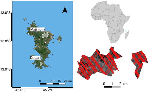
Table 1. List of the models used for the estimation of canopy heights and input data.

Model	Input data
MRH	rh_95 Slope Sensitivity
RFH	rh_n {10% ≤ n ≤ 100%, step 5%} Slope Sensitivity
sRFH	sim_RHT_n {10% ≤ n ≤ 100%, step 10%} sim_HG_n {10% ≤ n ≤ 100%, step 10%} Sensitivity

Figure 2. GEDI-CHM estimates from rh_100 (a), rh_98 (b) and rh_95 (c) as a function of ALS-CHM (als100).

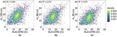
Table 2. Accuracy of GEDI-CHM estimates (rh_100, rh_98 and rh_95) against ALS-CHM (als100 and als95).

GEDI-CHM	Bias (m)	RMSE (m)
rh_100 vs. als100	2.1	7.4
rh_98 vs. als100	0.8	6.9
rh_95 vs. als100	−0.3	6.6
rh_95 vs. als95	3.9	7.5

Figure 3. CHM-Differences as a function of the difference between als100 and als95. The difference between als100 and als95 is an indicator of spatial heterogeneity.

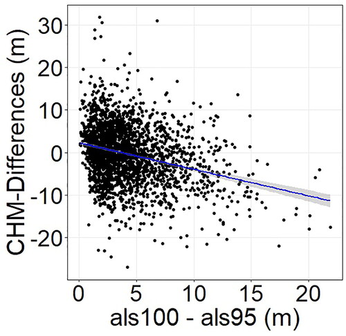
Figure 4. GEDI-CHM estimates (rh_95) as a function of als95 (a) and als100 (b).

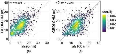
Figure 5. Boxplots of CHM-Differences depending on sensitivity class.

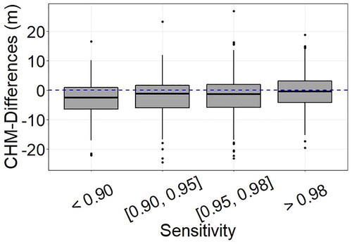
Table 3. Accuracy of GEDI-CHM estimates depending on beam sensitivity, tree height and mean slope.

	Bias (m)	RMSE (m)
Sensitivity
< 0.90	−3.2	7.3
[0.90, 0.95]	−2.3	6.6
[0.95, 0.98]	−1.8	6.5
> 0.98	−0.5	5.8
Tree height
< 15 m	0.6	4.7
> 15 m	−4.4	7.6
Slope
< 15°	1.1	4.8
[15°, 25°]	3.3	6.5
> 25°	5.9	9.4

Figure 6. CHM-Differences as a function of ALS-CHM (a) and boxplots of CHM-Differences depending on ALS-CHM class (b).

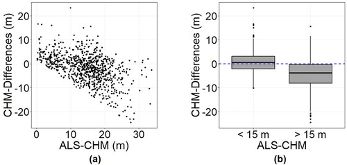
Figure 7. CHM-Differences as a function of slope (a) and boxplots of CHM-Differences depending on slope class (b).

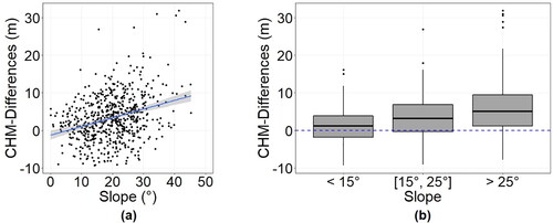
Figure 8. Boxplots of CHM-Differences depending on sensitivity class (a) and CHM-Differences as a function of slope (b) and ALS-CHM (c) for MRH and rh_95.

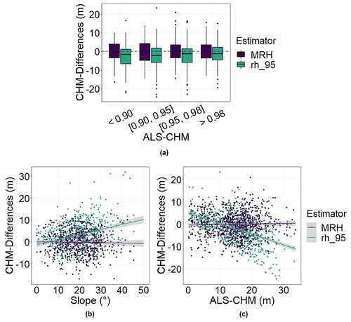
Table 4. Accuracy of GEDI-CHM estimates for rh_95 and the three regression models.

Estimator	Bias (m)	RMSE (m)	rRMSE
rh_95	−0.3	6.6	44%
MRH	0.0	5.7	38%
RFH	0.0	5.7	38%
sRFH	0.0	5.7	38%

Figure 9. Boxplots of CHM-Differences depending on sensitivity class (a) and CHM-Differences as a function of slope (b) and ALS-CHM (c) for RFH and rh_95.

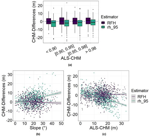
Figure 10. Boxplots of CHM-Differences depending on sensitivity class (a) and CHM-Differences as a function of slope (b) and ALS-CHM (c) for sRFH and rh_95.

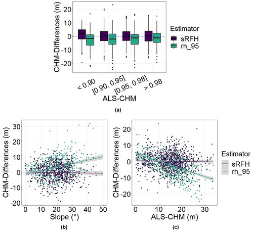
Figure 11. Importance of input variables (ten most important) using mean decrease Gini (%IncNodePurity) for RFH (a) and sRFH (b).

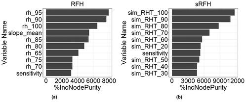
Figure 12. GEDI-CHM estimates from RFH (a) and sRFH (b) as a function of ALS-CHM.

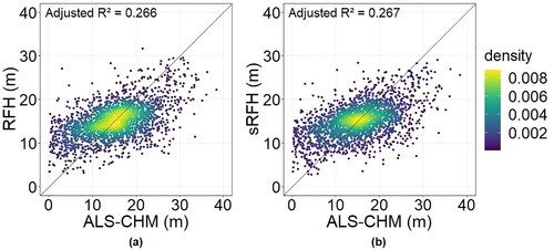
Figure 13. GEDI-CHM estimates as a function of ALS-CHM when using initial geolocations (a) and corrected geolocations (b).

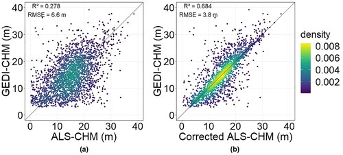
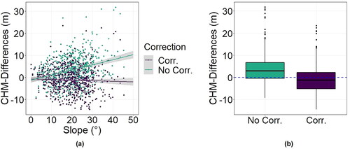
Figure 14. CHM-Differences as a function of slope (a) and boxplots of CHM-Differences (b) depending on whether a simple geometric correction is applied or not.