Figures & data
Fig. 1 The Bay of Fundy and Gulf of Maine with locations mentioned in the text indicated. The bathymetry contours are in metres.
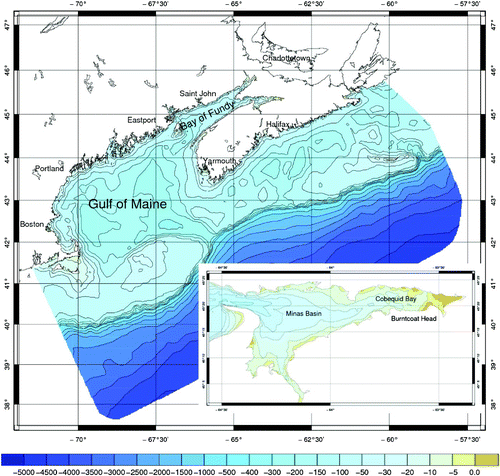
Fig. 2 Time series of the annual mean sea level (Z0) from analysis. The change in trend pre- and post-1980 was found to be statistically significant, as was a drop in mean sea level. The straight black lines show the trends and the coloured lines indicate the confidence intervals.
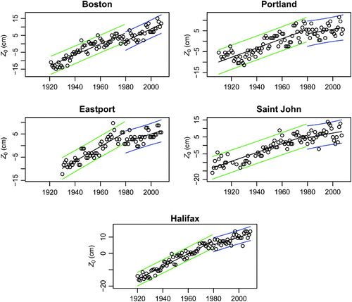
Fig. 3 The analyzed annual value of M2 amplitude showing the increasing trends in the Gulf of Maine and Bay of Fundy and the abrupt shift in value at 1982. The black curve is our fit to the data; the coloured curves are the 95% confidence intervals.
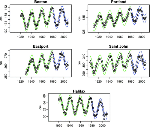
Fig. 4 Sea level rise per century as determined from the data analysis. The pre-break analyses from Boston, Portland, Saint John and Halifax are considered to be the most reliable.
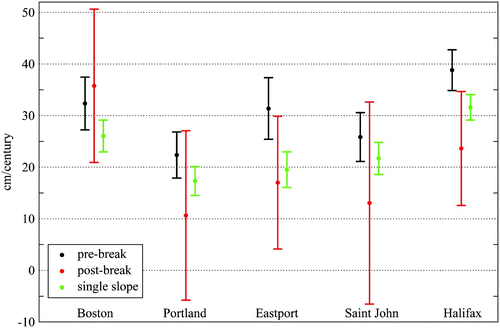
Table1. Tidal constituents analyzed. Frequencies are in cycles per hour.
Table 2. Estimated trends in Z0 and M2 tidal constituents with associated confidence intervals. The break in Z0 trend is at 1979/1980. The break in M2 amplitude and phase is at 1981/1982. Amplitude trends are in centimetres per century and phase trends are in degrees per century. The triples consist of lower confidence bound, point estimate of trend and upper confidence bound.
Table 3. Percentage change per century in amplitude. Triples consist of lower confidence bound, percentage change per century and upper confidence bound. Pre-1982 is percentage change per century pre-1982, relative to the 1970 predicted mean amplitude. Post-1981 is percentage change per century post-1981, relative to the 1982 predicted mean amplitude. Single slope is percentage change per century relative to the 1970 predicted mean amplitude.
Fig. 5 Change per century in M2 tidal amplitude as determined from the data analysis. The post-break Saint John line is off the scale (see and Section 2).
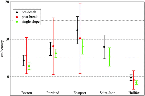
Fig. 6 Percentage change per century in M2 tidal amplitude. Note the proximity of the pre-break results from the Gulf of Maine and Bay of Fundy and the separation from Halifax. We believe this to be indicative of a phenomenon within the Gulf that is different from the adjacent surrounding ocean. Confidence bounds truncated by axis limits can be found in .
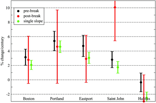
Fig. 7 Change per century in M2 tidal phase.
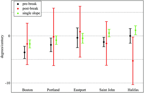
Fig. 8 The finite element model mesh used in tidal regime computations. There is higher resolution in shallow areas, in areas with steep gradients and in the Upper Bay of Fundy. The bathymetry colour scale is in metres.
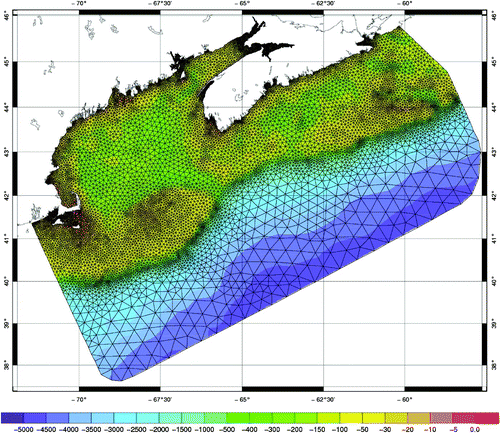
Fig. 9 Global average sea level rise 1990 to 2100 for the SRES scenarios. Thermal expansion and land-ice changes were calculated using a simple climate model calibrated separately for each of seven AOGCMs; contributions from changes in permafrost, the effect of sediment deposition and the long-term adjustment of the ice sheets to past climate change were added. Each of the six lines appearing in the key is the average of AOGCMs for one of the six illustrative scenarios. The region in dark shading shows the range of the average of AOGCMs for all thirty-five SRES scenarios. The region in light shading shows the range of all AOGCMs for all thirty-five scenarios. The region delimited by the outermost lines shows the range of all AOGCMs and scenarios including uncertainty in land-ice changes, permafrost changes and sediment deposition. Note that this range does not allow for uncertainty relating to ice-dynamic changes in the West Antarctic ice sheet (Figure 11.12 Church et al. (Citation2001)).
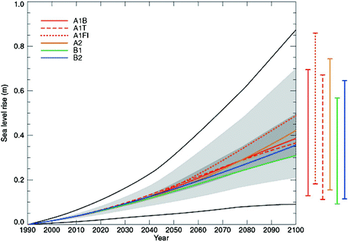
Fig. 10 Projections and uncertainties (5% to 95% ranges) of global average sea level rise and its components from 2090 to 2099 (relative to 1980 to 1999) for the six SRES marker scenarios (Figure 10.33 Meehl et al. (Citation2007)).
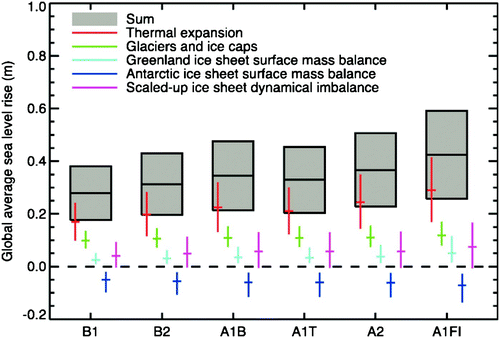
Fig. 11 Local sea level change (m) caused by ocean density and circulation change relative to the global average (i.e., positive values indicate greater local sea level change than global) during the twenty-first century, calculated as the difference between averages for 2070 to 2099 and 1980 to 1999, as an ensemble mean over 16 AOGCMs forced with the SRES A1B scenario. Stippling denotes regions where the magnitude of the multi-model ensemble mean divided by the multi-model standard deviation exceeds 1.0 (Figure 10.32 Meehl et al. (Citation2007)).
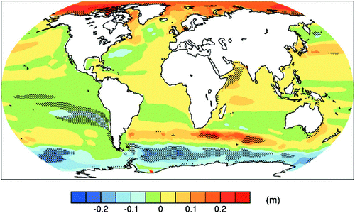
Table 4. Changes applied to model bathymetry (in metres) to account for cryospheric and steric effects on sea level. The ice changes are as derived in Section 5c, with values for 2055 and 2085 being obtained by linear interpolation. The steric sea level changes for 2055 and 2085 are taken from model runs analyzed for this study (Section 5b). The 2100 steric values were extrapolated from those computations.
Fig. 12 Our estimated pre-climate change rate of increase in sea level in metres per century. Named ports were specified from our analyses (Boston, Portland, Saint John and Halifax) and other publications (Newport, Woods Hole and Charlottetown). The values along the shelf break were set to 2.5 m during calibration to obtain agreement with the analyzed increase in M2 amplitude. Values on the deep sea open boundary were set to 0.4 metres per century. Other boundary values, needed to encompass the model domain, were specified to be consistent with nearby interior points. The increase in model bathymetry was linearly interpolated on the triangles of this mesh.
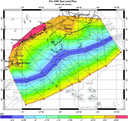
Fig. 13 Polar plot comparison between the calibrated model and the observations (red ▴). Radial variations correspond to differences in amplitude. Angular variations correspond to differences in phase.
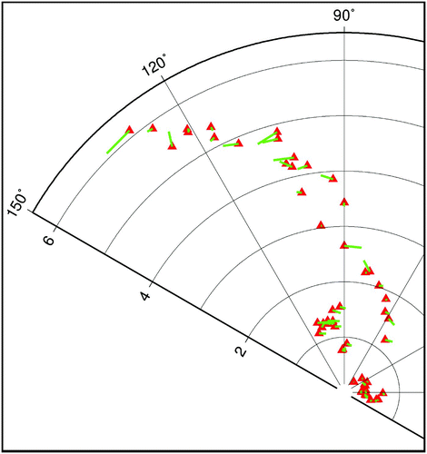
Fig. 14 Polar plot comparison between the calibrated model present state (red ▴) and the model predicted analyzed change (green line) and the existing change determined from the pre-break data analysis (blue line - see also ). Radial variations correspond to differences in amplitude in metres. Angular variations correspond to differences in phase.
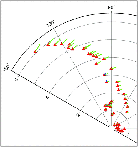
Fig. 15 Expanded scale for data analysis of the stations in . The stations shown, in order of increasing amplitude (radius), are Halifax, Portland (right), Boston (left), Eastport and Saint John.
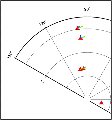
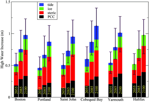
Fig. 16 The increase in the height of tidal high water from the sum of all factors as described in the text and the tables. PCC refers to the pre-climate change trends computed in Section 2. The error bar gives the maximum and minimum variation on this based on the literature for the ice contribution, the variability in the climate model results, and the tide computed taking into consideration these extremes.