Comparing Winter and Summer Simulated Estuarine Circulations in Foxe Basin, Canada

Figures & data

Fig. 1 Hudson Bay system (a) and Foxe Basin (b). In (a), the inset corresponds to Foxe Basin and its immediate neighbours. The model grid (partial, corresponding to the outputted data) is shown in (b); the star indicates the location of the mooring in Foxe Channel, the cross-section S is symbolized by the thick straight line, and the horizontal hatching shows the tidal flats area. The definitions of the acronyms are Baffin Bay (BB), Coats Island (CI), Foxe Basin (FB), Foxe Channel (FC), Fury and Hecla Strait (FHS), Foxe Peninsula (FP), Hall Beach (HaB), Hudson Bay (HB), Hudson Strait (HS), Lyon Inlet (LI), Melville Peninsula (MP), Mansel Islands (MI), Prince Charles Island (PCI), Repulse Bay (RB), Roes Welcome Sound (RWS) and Southampton Island (SI).

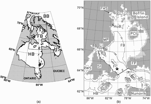
Fig. 2 Simulated ice growth rate averaged over Foxe Basin. The positive (negative) values correspond to the formation (melting) of sea ice.

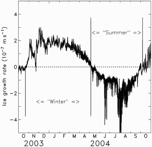
Fig. 3 Simulated ice growth rate averaged over the winter in Foxe Basin. The positive (negative) values correspond to the formation (melting) of sea ice. The vector field corresponds to the sea-ice velocity; its scale is given in the upper left box (see Fig. 1 for acronym definitions).

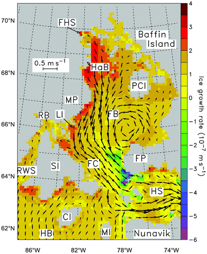
Fig. 4 Simulated sea-ice trajectory in Foxe Basin. The colour code of the tracers corresponding to the trajectories is given in the upper left box. In panels (a), (b) and (c), the run starts 1 November 2003, 1 February 2004 and 1 May 2004, respectively (see Fig. 1 for acronym definitions).

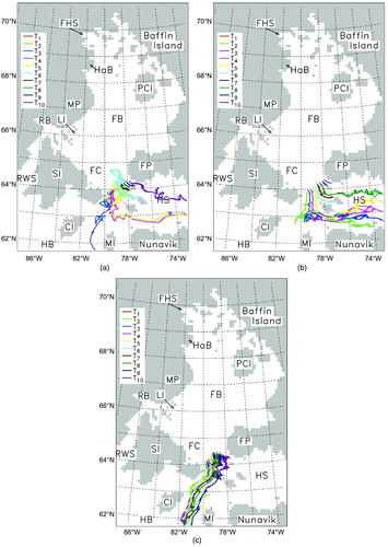
Table 1. Mean speed and total distance covered by the Lagrangian tracers leaving Foxe Basin (see Fig. 4 for trajectories). The dates indicate the start of each run (beginning of ice formation, maximum ice formation and beginning of ice melting). The last line contains the averaged speed for all tracers along with the standard deviation.

Tracer No.	1 November 2003		1 February 2004		1 May 2004
	Mean Speed (m s^−1)	Total Distance (km)	Mean Speed (m s^−1)	Total Distance (km)	Mean Speed (m s^−1)	Total Distance (km)
T1	0.18	17	0.01	0	0.02	0
T2	0.14	233	0.16	2428	0.13	994
T3	0.19	837	0.19	2586	0.15	1168
T4	0.26	1135	0.21	1353	0.16	1237
T5	0.32	1465	0.23	1218	0.17	1283
T6	0.40	1601	0.11	389	0.18	1367
T7	0.29	180	0.20	320	0.19	1340
T8	0.15	79	0.27	1404	0.20	1379
T9	0.11	95	0.16	89	0.21	1349
T10	0.19	935	0.13	87	0.25	759
Speed (m s^−1)	0.22 ± 0.10		0.17 ± 0.08		0.17 ± 0.07

Fig. 5 Simulated temperature (panels (a), (c), (e), (g)), salinity (panels (b), (d), (f), (h)) and seawater velocity fields (panels (a)–(h)), averaged over winter and summer in Foxe Basin. The velocity scale is given in the upper left box. (a) and (b) correspond to the winter surface fields; (c) and (d) to the winter bottom fields; (e) and (f) to the summer surface fields; and (g) and (h) to the summer bottom fields. In order to ease the reading of the figures, the velocity field is the same in (a) and (b), (c) and (d), (e) and (f), and (g) and (h). Note that, in (c), (d), (g) and (h), the fields are, in fact, calculated near the bottom because they correspond to the middle of the deepest grid cells (see Fig. 1 for acronym definitions).

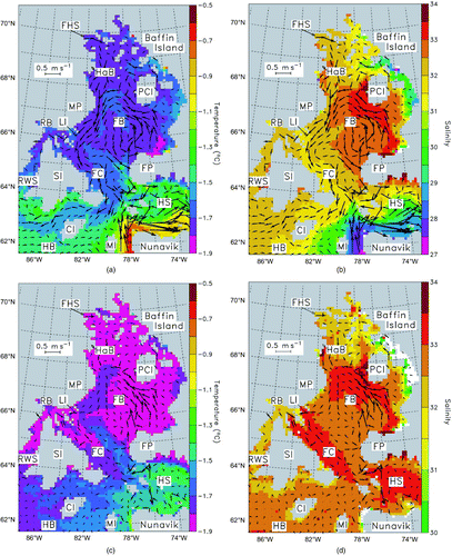
Fig. 5 Concluded

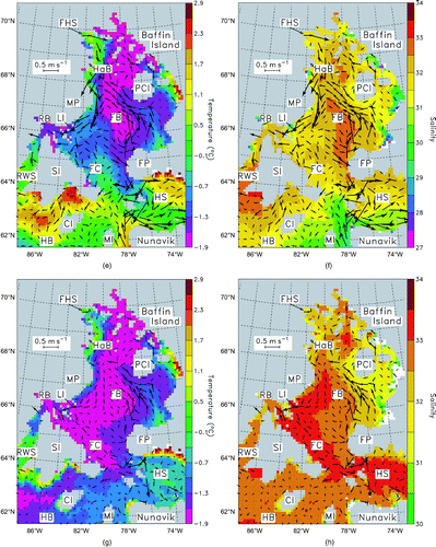
Fig. 6 Simulated temperature (a) and salinity (b) and the comparison between simulated and observed temperature (c) profiles versus depth in Foxe Channel. The location of the profiles corresponds to the mooring deployed at 64.37°N and 80.55°W from August 2004 to August 2005 (see Fig. 1b). In (a) and (b), the solid and dashed lines represent the winter and summer, respectively. In (c), the circles correspond to the observations and the solid line to the simulated data averaged over the period matching the time series.

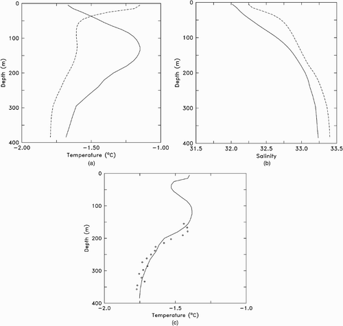
Fig. 7 Simulated sea-ice thickness averaged over the winter in Foxe Basin (see Fig. 1 for acronym definitions and Fig. 3 for the vector field description).

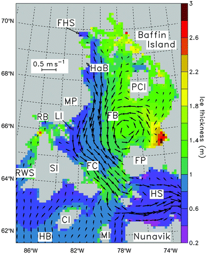
Fig. 8 Satellite image taken 20 June 2002 over Foxe Basin and its surrounding parts (copyright NASA, 2008). The significance of the arrows is given in Section 4.a.

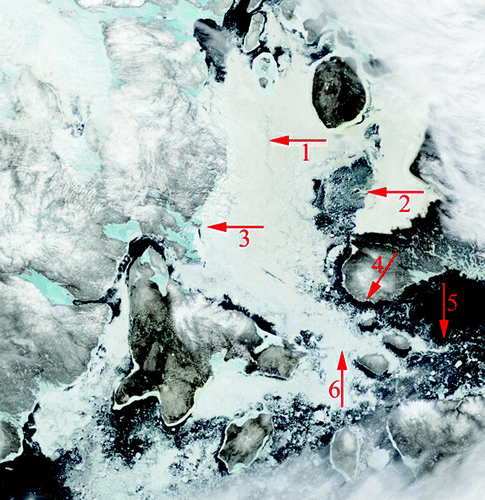
Fig. 9 Vertical simulated seawater (a) and salt (b) transport through cross-section S in Foxe Channel (see Fig. 1b). The solid and dashed lines correspond to the winter and summer, respectively. In (a) and (b), the transport is calculated through 10 m thick layers on S from the surface to the bottom of the channel. In (a), negative (positive) values indicate an output (input) stream; in (b), the salt transport anomaly is defined as the difference between the salinity measured at the section and the mean salinity in Foxe Basin.

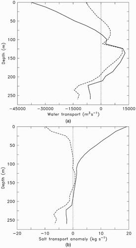
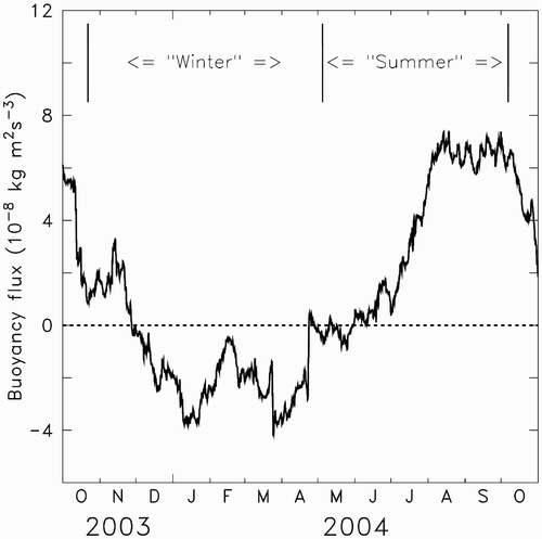
Fig. 10 Mean vertical buoyancy flux in Foxe Basin (see Section 3.a and Fig. 2 for the winter and summer definitions).

NASA. 2008 Visible Earth. Retrieved from http://visibleearth.nasa.gov/view.php?id=60255

 Google Scholar