Simulating the Carbon Cycling of Northern Peatlands Using a Land Surface Scheme Coupled to a Wetland Carbon Model (CLASS3W-MWM)

Figures & data

Fig. 1 The basic coupling structure of the coupled land surface climate model (CLASS3W) and the peatland C model (MWM) (referred as CLASS3W-MWM).

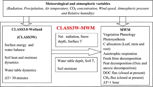
Table 1. The detailed physical characteristics and mean climate conditions for the two evaluation peatlands.

Characterstics	Bog (MB)	Fen (DS)
Name	Mer Bleue	Degerö Stormyr
Location	45.41°N, 75.48°W, eastern Canada	64°11′N, 19°33′E, northern Sweden
Climate	Cool continental temperate	Cold temperate humid
Peatland classification	Ombrotrophic bog	Minerotrophic poor fen
Nutrients	Poor	Rich
Water sources	Precipitation	Precipitation, surface runoff and groundwater
Size	28 km^2	6.5 km^2
Depth of peat	5–6 m	3–4 m
Basal age	approximately 9000 years	approximately 8000 years
Dominant plants	Moss and shrubs	Moss and sedges
Surface topography	69 m above mean sea level	270 m above mean sea level
Mean annual Ta (°C)	6.0	1.2
Monthly max. Ta (°C)	20.9	14.7
Monthly min. Ta (°C)	−10.8	−12.4
Days above 0°C	206.0	150.0
Mean annual P (mm)	943.0	523.0
Precipitation as snow (mm)	235.0	233.0
Monthly max. P (mm)	90.0	65.0
Monthly min. P (mm)	60.0	25.0
Note: MB denotes Mer Bleue and DS denotes Degerö Stormyr.

Table 2. Parameters and initial values used in CLASS3W-MWM for MB and DS.

Parameter	Bog (MB)	Fen (DS)	Units	Description	Reference/Source
Values for Model Parameters at 25°C
J max:V max	1.67	1.67	—	ratio	(Medlyn et al., 2002)
Mosses
V cmax25	6	6.5	μmol m^−2 s^−1	max carboxylation rate (spring)
	14	14	μmol m^−2 s^−1	max carboxylation rate (summer)
	7	7.5	μmol m^−2 s^−1	max carboxylation rate (autumn)
R d25	0.946	0.946	μmol m^−2 s^−1	dark respiration rate	(Harley et al., 1986)
Shrubs/Sedges
V cmax25	17	20	μmol m^−2 s^−1	max carboxylation rate
Initial site specific parameters
frac	48.7	48.7	%	biomass to carbon ratio
B moss	140	150	g biomass m^−2	moss capitula biomass
B min foliar	175	90	g biomass m^−2	min shrub/sedge foliar biomass
B max foliar	350	180	g biomass m^−2	max shrub/sedge foliar biomass
LAI_moss	1.35	1.05	m^2/m^2	initial moss leaf area index
LAI_shrub/sedge	0.9	0.5	m^2/m^2	initial shrub/sedge leaf area index
Root_shrub/sedge	500	450	g biomass m^−2	Initial shrub/sedge root biomass
Litter_shrub/sedge	150	250	g biomass m^−2	Initial shrub/sedge litter biomass
B stem	0.003		m^3 m^−2	shrub sapwood volume
PD0	6	4	m	initial peat depth
k o	0.05/0.2	0.05/0.2	yr^−1	initial decomposition rate for moss/shrub(sedge)	(Frolking et al., 2001)
Initial values for organic soil
Z	0.20/0.75/6.0	0.20/0.75/4.0	m	Depth to bottom of 3 soil layers	(Ouyang et al., in press)
θp	0.93/0.88/0.83	0.93/0.88/0.83		Porosity for 3 soil layers	(Letts et al., 2000)
θr	0.175/0.530/0.705	0.175/0.530/0.705		Specific retention for 3 soil layers	(Letts et al., 2000)
θm	0.04/0.15/0.22	0.04/0.15/0.22		Residual soil water content for 3 soil layers	(Letts et al., 2000)
b	2.7/6.1/9.5	2.7/6.1/9.5		Soil texture parameter	(Letts et al., 2000)
Ψs	9.6 × 10^−3/9.06 × 10^−3/8.3 × 10^−3	9.6 × 10^−3/9.06 × 10^−3/8.3 × 10^−3	m	Soil matric potential at saturation	(Ouyang et al., in press)
γ	1.7 × 10^−4/2.0 × 10^−6/1. × 10^−8	1.7 × 10^−4/2.0 × 10^−6/1.0 × 10^−8	m s^−1	Hydraulic conductivity at saturation	(Ouyang et al., in press)

Fig. 2 80-year simulation of (a) water table depth (WTD) and (b) the temperature of the first soil layer (soil1_T) based on the 10 repeated simulations of 1999–2006 for Mer Bleue (MB).

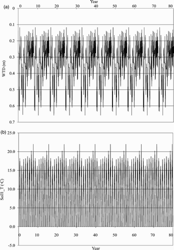
Fig. 3 Comparison of CLASS3W-MWM simulated summer WTD and the temperature of the first soil layer (soil1_T) with observations for MB ((a) and (b)) and Degerö Stormyr (DS) ((c) and (d)). The regression equation and r ² are also shown. Note: The black line in the graph is the perfect 1:1 line.

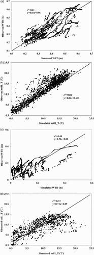
Table 3. CLASS3W-MWM simulated and observed annual GPP (GPP_M, GPP_O), TER (TER_M, TER_O), NEP (NEP_M, NEP_O) for MB; and the annual NPP and the percentage contribution of each simulated component. The suffix “O” represents observed fluxes and “M” represents simulated fluxes. The 8-year average (Ave) is also shown. For comparison, the stand-alone MWM simulated fluxes (GPP_MO, TER_MO, NEP_MO), based on observed soil temperature and WTD, are also presented (reproduced from St-Hilaire et al. (2010)). The anomalies of annual average air temperature (ΔT) and precipitation (ΔP), relative to the 8-year average value (Ave), are shown.

Year	GPP					TER							NEP			NPP
	GPP_O	GPP_M	GPP_MO	Moss	Shrub	TER_O	TER_M	TER_MO	AR	MossAR	ShrubAR	HR	NEP_O	NEP_M	NEP_MO	NPP_M	Moss	Shrub	ΔT	ΔP
	g C m^−2 yr^−1	g C m^−2 yr^−1	g C m^−2 yr^−1	%	%	g C m^−2 yr^−1	g C m^−2 yr^−1	g C m^−2 yr^−1	%	%	%	%	g C m^−2 yr^−1	g C m^−2 yr^−1	g C m^−2 yr^−1	g C m^−2 yr^−1	%	%	°C	mm
1999	646.2	607.0	624.0	42.5	57.5	−581.7	−466.3	−623.0	73.8	25.1	48.7	26.2	64.6	140.7	1.0	262.9	53.7	46.3	0.6	6.9
2000	463.2	568.7	628.0	45.1	54.9	−431.3	−475.9	−550.0	71.2	28.1	43.1	28.8	31.9	92.8	78.0	229.8	53.5	46.5	−0.9	−129.9
2001	543.3	638.5	662.0	42.5	57.5	−541.3	−496.4	−623.0	71.4	24.0	47.3	28.6	2.0	142.1	39.0	284.2	53.4	46.6	0.6	−200.1
2002	511.0	595.3	647.0	43.6	56.4	−498.1	−501.4	−612.0	70.1	25.9	44.2	29.9	12.9	93.9	35.0	244.0	53.1	46.9	0.2	−54.3
2003	494.6	592.2	667.0	40.8	59.2	−480.2	−521.9	−582.0	73.3	26.9	46.3	26.7	14.4	70.4	85.0	209.9	48.2	51.8	−1.0	−11.1
2004	683.0	619.3	713.0	41.2	58.8	−567.8	−517.9	−580.0	75.5	28.3	47.1	24.5	115.2	101.4	133.0	228.5	47.5	52.5	−0.9	167.1
2005	688.3	632.3	710.0	38.7	61.3	−597.9	−566.1	−609.0	75.9	27.6	48.3	24.1	90.4	66.2	101.0	202.7	43.6	56.4	0.1	19.5
2006	772.2	628.2	704.0	39.8	60.2	−624.7	−556.8	−604.0	76.9	28.8	48.0	23.1	147.5	71.4	99.0	200.2	44.8	55.2	1.0	201.9
Ave	600.2	610.2	669.4	41.8	58.2	−540.4	−512.8	−597.9	73.5	26.9	46.6	26.5	59.9	97.4	71.4	232.8	49.7	50.3	6.2	660.9
Note: For air temperature anomalies, negative indicates colder and positive warmer temperatures. For precipitation anomalies, negative indicates drier and positive indicates wetter conditions.

Table 4. CLASS3W-MWM simulated GPP (GPP_M), TER (TER_M), NEP (NEP_M), NPP (NPP_M) and observed NEP (NEP_O), and the percentage contribution of each simulated component for DS. The suffix “O” represents observed fluxes and “M” represents simulated fluxes. The 6-year average (Ave) is also shown. For comparison, the stand-alone MWM simulated fluxes (GPP_MO, TER_MO, NEP_MO), based on observed soil temperature and WTD, are also presented (Wu et al., unpublished manuscript). The annual average air temperature anomalies (ΔT) and precipitation anomalies (ΔP), relative to the 6-year average value (Ave), are shown.

Year	GPP				TER						NEP			NPP
	GPP_M	GPP_MO	Moss	Sedge	TER_M	TER_MO	AR	MossAR	SedgeAR	HR	NEP_O	NEP_M	NEP_MO	NPP_M	Moss	Sedge	ΔT	ΔP
	g C m^−2 yr^−1	g C m^−2 yr^−1	%	%	g C m^−2 yr^−1	g C m^−2 yr^−1	%	%	%	%	g C m^−2 yr^−1	g C m^−2 yr^−1	g C m^−2 yr^−1	g C m^−2 yr^−1	%	%	°C	mm
2001	443.2	394.0	36.8	63.2	357.6	344.0	73.2	18.6	54.6	26.8	47.9	85.6	50.0	181.4	53.1	46.9	0.1	162.8
2002	494.8	593.0	29.9	70.1	467.5	532.0	68.5	17.5	51.0	31.5	60.6	27.3	61.0	174.4	37.9	62.1	0.7	58.0
2003	370.6	455.0	35.1	64.9	260.6	405.0	81.9	28.9	53.0	18.1	59.1	110.0	50.0	157.1	34.8	65.2	0.0	105.2
2004	245.1	353.0	35.9	64.1	236.8	313.0	78.8	20.5	58.3	21.2	54.9	8.3	40.0	58.4	67.6	32.4	−2.6	−14.0
2005	490.5	477.0	29.9	70.1	458.0	427.0	71.2	18.0	53.2	28.8	47.5	32.5	50.0	164.2	39.1	60.9	1.3	−60.8
2006	381.9	419.0	35.3	64.7	354.7	404.0	63.7	15.9	47.8	36.3	17.3	27.2	15.0	155.9	50.4	49.6	0.7	−251.2
Ave	404.3	449.0	33.8	66.2	355.9	404.0	72.9	19.9	53.0	27.1	47.9	48.5	44.0	148.6	47.2	52.8	2.3	568.0
Note: For air temperature anomalies, negative indicates colder and positive indicates warmer temperatures. For precipitation anomalies, negative indicates drier and positive indicates wetter conditions.

Fig. 4 Temporal trend and comparison of daily observed and CLASS3W-MWM simulated GPP (top panel), TER (middle panel) and NEP (bottom panel) for 1999–2006 for MB (the filled black circles show the observed CO₂ fluxes, and the open red circles show the CLASS3W-MWM simulated CO₂ fluxes).

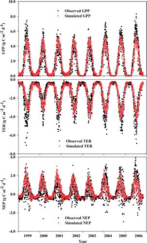
Fig. 5 Temporal trend and comparison of daily observed and CLASS3W-MWM simulated NEP for 2001–06 for DS (the filled black circles show the observed NEP, and the open red circles show the CLASS3W-MWM simulated NEP).

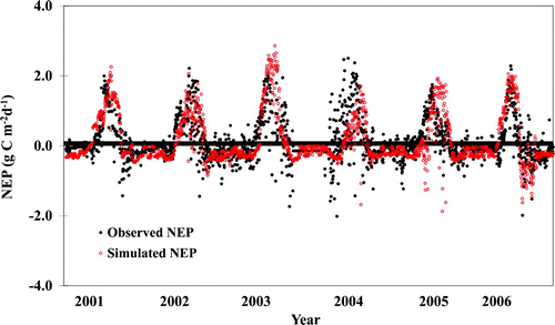
Fig. 6 The 1:1 scatterplots of observed and CLASS3W-MWM simulated daily GPP and TER for MB for 1999–2006. The solid black line is the perfect 1:1 line. The filled circles show the GPP, and the open circles show the TER. The regression equation r ², d*, and the RMSE are also shown.

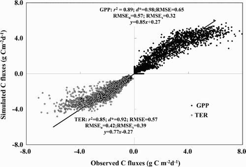
Fig. 7 The 1:1 scatterplots of observed and CLASS3W-MWM simulated daily NEP for MB for 1999–2006 (top panel) and DS for 2001–06 (bottom panel). The solid black line is the perfect 1:1 line. The regression equation r ², d*, and the RMSE are also shown.

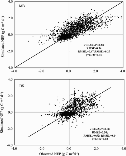
Table 5. Sensitivity of CLASS3W-MWM simulated GPP, AR, NPP , NEP, TER, OxicHR and AnoxicHR to changes in air temperature (T_a ), precipitation (P), atmospheric CO₂ concentration ([CO₂]) and combinations of these, expressed as a relative change in percentage of the base line fluxes, for Mer Bleue (MB) (a) and Degerö Stormyr (DS) (b). Negative percentage changes indicate a decrease, and positive percentage changes indicate an increase relative to the base line value. The percentage change is calculated by “(new value-base line)/base line × 100”. The baseline C fluxes were calculated based on CLASS3W-MWM using present-day climate inputs. Changes in T_a were imposed by its absolute changed values, whereas changes in precipitation were imposed by its relative changed percentage. Positive changes in T_a indicate warmer temperatures, and negative changes in T_a indicate cooler temperatures. Negative changes in precipitation indicate decreased precipitation, and positive changes indicate increased precipitation. Only doubled atmospheric CO₂ concentration was applied (2 × CO₂). Care should be taken that the changes were evenly distributed in the study period. The last three columns show the absolute C fluxes for GPP, TER and NEP when those changes were imposed.

	Base line (g C m^−2 yr^−1)	Moss (%)			Shrub (%)			HR (%)		Total (%)			Total	gC m^−2 yr^−1
		GPP	AR	NPP	GPP	AR	NPP	Oxic HR	Anoxic HR	NEE	TER	GPP	NEE	TER	GPP
		254.7	138.0	116.7	355.5	239.5	116.0	122.9	12.5	97.4	512.8	610.2	97.4	512.8	610.2
(a) For MB
	Ta (−3)	−10.8	−16.7	−3.9	−21.3	−14.2	−35.8	−19.8	−26.1	−18.9	−16.5	−16.9	78.9	428.2	507.1
	Ta (−2)	−7.1	−9.0	−4.7	−13.9	−9.1	−24.0	−12.8	−7.1	−17.3	−9.9	−11.1	80.6	462.1	542.7
	Ta (−1)	−3.0	−2.5	−3.5	−6.7	−4.5	−11.3	−6.3	−1.4	−9.5	−4.3	−5.2	88.1	490.6	578.7
T	Ta (+1)	−1.6	2.8	−6.8	6.2	6.2	6.1	5.9	7.5	−9.5	5.3	2.9	88.2	539.9	628.1
	Ta (+2)	−6.5	5.7	−21.0	12.0	13.4	9.1	9.9	12.8	−28.5	10.5	4.3	69.6	566.6	636.2
	Ta (+3)	−11.2	6.0	−31.5	16.3	23.6	1.4	16.1	22.3	−59.3	17.0	4.9	39.6	600.3	639.9
	Ta (+5)	−29.0	−2.1	−60.8	22.7	40.8	−14.7	31.1	29.3	−133.4	26.7	1.1	−32.5	649.7	617.2
	P(−30%)	−21.5	−30.6	−10.8	0.2	−1.1	2.9	11.1	12.8	−25.2	−5.8	−8.9	72.8	483.2	556.0
	P(−20%)	−7.6	−14.0	−0.050	0.1	−1.0	2.3	4.7	10.0	−4.7	−2.8	−3.1	92.8	498.3	591.1
P	P(−10%)	−1.4	−5.7	3.8	0.037	−0.4	0.9	2.4	6.4	1.6	−1.0	−0.5	99.0	507.9	606.9
	P(+10%)	0.024	4.7	−5.5	−0.025	0.3	−0.7	−1.9	−4.3	−4.4	0.8	−0.005	93.1	517.1	610.2
	P(+20%)	−0.3	7.8	−9.8	−0.041	0.8	−1.8	−3.2	−18.0	−7.5	1.3	−0.1	90.1	519.3	609.4
	P(+30%)	−0.5	9.9	−12.7	−0.1	1.2	−2.7	−4.0	−20.7	−10.8	1.8	−0.2	86.8	522.0	608.8
CO2	2 CO2	15.4	0.0	33.6	37.2	21.1	70.4	35.3	0.045	79.6	18.3	28.1	174.9	606.9	781.7
T+P	2 + (+30%)	0.5	23.6	−26.9	11.9	14.6	6.2	4.3	2.9	−30.6	14.3	7.1	67.6	586.0	653.6
	3 + (+30%)	0.1	30.0	−35.4	16.2	20.8	6.8	7.5	6.2	−44.6	19.7	9.5	53.9	614.1	668.0
	5 + (+30%)	−0.8	43.2	−52.9	22.5	39.7	−13.2	18.0	15.7	−103.9	34.9	12.7	−3.8	691.8	688.0
	2 + (−30%)	−48.0	−46.2	−50.2	12.3	16.4	3.7	66.6	18.4	−142.2	11.7	−12.9	−41.0	572.6	531.6
	3 + (−30%)	−59.5	−56.4	−63.3	17.1	23.9	3.0	79.5	20.5	−175.3	15.6	−14.9	−73.3	592.7	519.4
	5 + (−30%)	−85.5	−84.9	−86.3	24.7	47.6	−22.7	289.6	−14.6	−494.2	68.5	−21.3	−383.9	863.9	480.1
T + P +  CO2	2 + (+30%) + 2 CO2	16.8	23.6	8.9	54.8	42.5	80.2	43.2	2.9	51.2	36.6	39.0	147.3	700.7	848.0
	3 + (+30%) + 2 CO2	16.9	30.0	1.5	61.6	54.1	77.1	49.4	6.2	30.4	45.4	43.0	127.0	745.4	872.4
	5 + (+30%) + 2 CO2	16.9	43.2	−14.2	72.0	77.9	59.7	61.7	15.7	−25.8	63.2	49.0	72.3	836.9	909.2
	2 + (−30%) + 2 CO2	−39.7	−46.2	−31.9	55.0	44.4	76.9	101.0	18.4	−76.6	33.0	15.5	22.8	682.0	704.8
	3 + (−30%) + 2 CO2	−52.8	−56.4	−48.5	62.1	57.2	72.2	115.5	20.5	−120.6	39.7	14.1	−20.0	716.5	696.5
	5 + (−30%) + 2 CO2	−83.0	−84.9	−80.7	73.2	83.5	52.1	323.7	−14.6	−441.5	93.4	8.0	−332.6	991.8	659.3
	Base line (g C m^−2 yr^−1)	Moss (%)			Sedget (%)			HR (%)		Total (%)			Total	gC m^−2 yr^−1
		GPP	AR	NPP	GPP	AR	NPP	Oxic HR	Anoxic HR	NEE	TER	GPP	NEE	TER	GPP
		157.8	71.1	86.7	322.3	224.5	97.8	100.0	20.7	63.9	416.3	480.1	63.9	416.3	480.1
(b) For DS
	Ta (−3)	−7.8	−27.4	8.4	−28.6	−21.7	−44.4	−27.1	−14.3	−9.6	−23.6	−21.8	57.7	317.9	375.7
	Ta (−2)	−7.0	−18.7	2.7	−18.6	−13.9	−29.4	−15.7	−5.3	−15.3	−14.7	−14.8	54.1	355.0	409.1
	Ta (−1)	1.1	−9.6	9.9	−7.3	−4.4	−13.8	−5.4	−7.4	3.0	−5.7	−4.5	65.8	392.6	458.4
T	Ta (+1)	−1.5	12.6	−13.1	6.8	−1.5	25.7	9.9	−13.2	10.3	3.1	4.0	70.4	429.1	499.5
	Ta (+2)	−14.7	13.3	−37.6	−1.5	−2.9	1.5	32.3	−23.0	−91.9	7.3	−5.9	5.2	446.8	452.0
	Ta (+3)	−35.2	−5.2	−59.8	−17.5	−8.2	−38.7	48.3	−46.6	−200.9	4.0	−23.3	−64.4	432.7	368.3
	Ta (+5)	−48.1	−28.2	−64.5	−38.2	−3.9	−116.9	152.1	−61.2	−485.0	26.6	−41.4	−245.9	527.0	281.1
	P(−30%)	5.8	3.3	7.9	2.1	−5.4	19.4	−4.5	−16.2	52.8	−4.3	3.3	97.6	398.5	496.1
	P(−20%)	7.2	1.5	11.9	2.9	−4.0	18.7	−6.1	−16.9	59.8	−4.2	4.3	102.0	398.8	500.8
P	P(−10%)	4.9	0.7	8.3	1.4	−2.1	9.4	−3.0	−9.4	33.5	−2.2	2.5	85.2	407.0	492.3
	P(+10%)	−1.4	−0.2	−2.4	−1.6	−0.8	−3.4	−1.6	−3.6	−4.8	−1.0	−1.5	60.8	412.1	472.9
	P(+20%)	−3.6	−0.047	−6.5	−3.6	−2.4	−6.3	−3.2	−5.0	−11.8	−2.3	−3.6	56.3	406.6	462.9
	P(+30%)	−3.2	−0.027	−5.8	−2.9	−2.0	−5.1	−2.8	−3.9	−10.0	−1.9	−3.0	57.5	408.2	465.7
CO2	2 CO2	12.3	0.000	22.4	23.5	11.3	51.5	37.9	−13.8	54.4	14.5	19.8	98.6	476.7	575.3
T + P	2 + (+30%)	1.2	25.6	−18.8	14.1	6.5	31.4	21.0	−9.6	−7.3	12.5	9.8	59.2	468.1	527.3
	3 + (+30%)	−15.1	17.3	−41.6	5.5	4.7	7.3	45.1	−18.8	−109.9	15.4	−1.3	−6.3	480.2	473.9
	5 + (+30%)	−31.8	−1.0	−57.0	−6.4	5.3	−33.2	102.9	−40.0	−276.4	25.4	−14.7	−112.7	522.1	409.4
	2 + (−30%)	−40.9	−28.9	−50.8	−25.8	−24.3	−29.3	16.0	−58.1	−120.1	−17.1	−30.8	−12.8	345.2	332.4
	3 + (−30%)	−68.1	−66.6	−69.3	−44.0	−30.1	−75.9	96.8	−86.8	−333.8	−8.7	−51.9	−149.3	380.2	230.9
	5 + (−30%)	−81.8	−77.6	−85.3	−42.1	−19.3	−94.4	250.6	−78.5	−627.3	32.6	−55.2	−336.8	552.1	215.3
T + P + CO2	2 + (+30%) + 2 CO2	13.8	25.6	4.1	43.4	20.8	95.1	62.6	−24.3	61.1	29.4	33.6	102.9	538.8	641.7
	3 + (+30%) + 2 CO2	−4.1	17.3	−21.6	32.3	19.0	62.9	82.4	−29.5	−52.5	31.5	20.3	30.3	547.4	577.7
	5 + (+30%) + 2 CO2	−22.2	−1.0	−39.5	15.8	17.4	12.0	138.2	−52.6	−234.6	39.8	3.3	−86.0	581.9	495.9
	2 + (−30%) + 2 CO2	−33.5	−28.9	−37.3	−10.1	−17.0	6.0	36.6	−63.9	−78.0	−8.5	−17.8	14.1	380.8	394.9
	3 + (−30%) + 2 CO2	−64.3	−66.6	−62.3	−35.7	−25.3	−59.5	102.1	−86.7	−307.6	−4.8	−45.1	−132.6	396.2	263.6
	5 + (−30%) + 2 CO2	−80.0	−77.6	−81.9	−38.4	−16.9	−87.9	254.6	−80.2	−618.4	34.8	−52.1	−331.1	561.1	230.1
The notation is P(−30%) indicates a decrease in P of 30%; Ta (−3) indicates a decrease in Ta of 3°C; 2 CO2 inidcates doubled CO2 concentration; 2+(+30%) inidcates a combination of an increase in Ta of 2°C and an increase in P of 30%; 2+(+30%) + 2 CO2 indicates a combination of an increase in Ta of 2°C, an increase in P of 30% and doubled CO2 concentration.

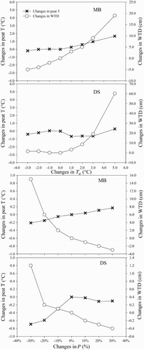
Fig. 8 The changes in peat temperature (T: °C) and WTD (cm) relative to the baseline simulated peat temperature and WTD responding to changes in air temperature (T_a : °C) (top two panels) and changes in precipitation (P: %) (bottom two panels). Note: (1) Positive changes in peat temperature indicate an increase, and negative changes indicate a decrease; positive changes in WTD indicate an increase (or drier conditions), and negative changes indicate a decrease (or wetter conditions). (2) Different scales are used for changes in WTD for MB and DS.

Medlyn , B. E. , Dreyer , E. , Ellsworth , D. , Forstreuter , M. , Harley , P. C. , Kirschbaum , M. U.F. , Le Roux , X. , Montpied , P. , Strassemeyer , J. , Walcroft , A. , Wang , K. and Loustau , D. 2002 . Temperature response of parameters of a biochemically based model of photosynthesis, II, A review of experimental data . Plant, Cell Environ. , 25 : 1167 – 1179 . doi:10.1046/j.1365-3040.2002.00891.x

 Web of Science ®Google Scholar

Harley , P. C. , Tenhunen , J. D. and Lange , O. L. 1986 . Use of an analytical model to study limitations on net photosynthesis in Arbutus unedo under field conditions . Oecologia , 70 : 393 – 401 . (doi:10.1007/BF00379502)

 Web of Science ®Google Scholar

Frolking , S. , Roulet , N. T. , Moore , T. R. , Richard , P. J.H. , Lavoie , M. and Muller , S. D. 2001 . Modeling northern peatland decomposition and peat accumulation . Ecosystems , 4 ( 5 ) : 479 – 498 . (doi:10.1007/s10021-001-0105-1)

 Web of Science ®Google Scholar

Ouyang , B. , Roulet , N. T. , Lafleur , P. M. and Verseghy , D. in press . Modelling the water table in bogs using the Canadian Land Surface Scheme (CLASS) . Hydrol. Processes ,

 Google Scholar

Letts , M. G. , Roulet , N. T. , Comer , N. T. , Skarupa , M. R. and Verseghy , D. 2000 . Parameterization of peatland hydraulic properties for the Canadian Land Surface Scheme . Atmosphere-Ocean , 38 ( 1 ) : 141 – 160 . (doi:10.1080/07055900.2000.9649643)

 Web of Science ®Google Scholar

St-Hilaire , F. , Wu , J. , Roulet , N. T. , Frolking , S. , Lafleur , P. M. , Humphreys , E. and Arora , V. 2010 . McGill Wetland Model: Evaluation of a peatland carbon simulator developed for global assessments . Biogeosciences, , 7 : 3517 – 3530 . doi:10.5194/bg-7-3517-2010

 Web of Science ®Google Scholar