Circulation Around Luzon Strait in September as Inferred from CTD, Argos and Argo Measurements and a Generalized Topography-Following Ocean Model

Figures & data

Fig. 1 (a) Bottom topography (m) around Luzon strait. (b) Observation stations of the survey from 31 August to 10 September 1994 as well as the horizontal grid of the model used.

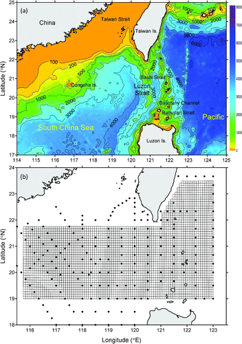
Fig. 2 Temperature distributions at (a) the surface, (b) 200 m and (c) 500 m depths obtained from 31 August to 10 September 1994.

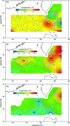
Fig. 3 Wind stress derived from National Centers for Environmental Prediction (NCEP) reanalysis data for the survey period.

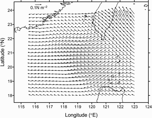
Fig. 4 Depth (m) distributions for the (a) 25.0 and (b) 26.0 isopycnal surfaces in September 1994. The arrows indicate the current direction.

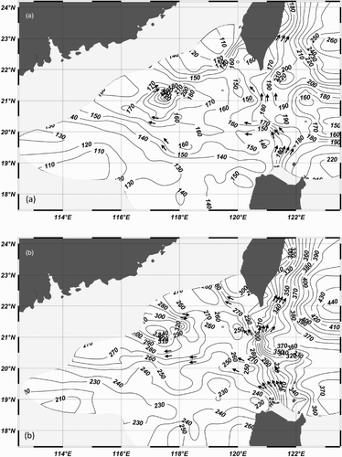
Fig. 5 Half-degree averaged drifter velocities for September (a) between 1 July 1989 and 30 June 2010 and (b) from 1990 to 2005.

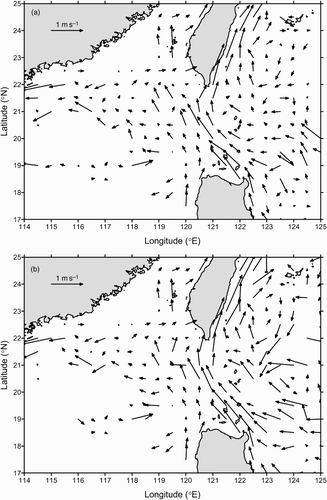
Fig. 6 Trajectories of Argo drifters appearing in September between 26 September 2002 and 30 January 2010. The blue dots denote their initial positions in September, and the numbers indicate their parking levels (m).

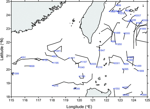
Fig. 7 Vertical coordinates in a west–east cross-section along 20.5°N. (a) The GTF coordinate grid and (b) the conventional σ coordinate grid.

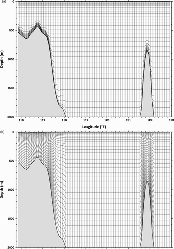
Fig. 8 Horizontal velocity distributions for diagnostic calculation at (a) the surface, (b) 200 m, (c) 500 m and (d) 1000 m depths.

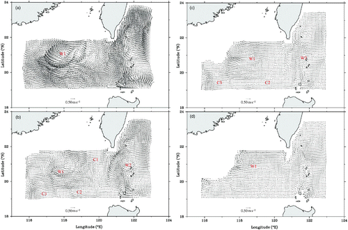
Fig. 9 Velocity distributions (cm s⁻¹) from ADCP current observations at 40 m depth from 28 August to 10 September 1994 (one degree latitude corresponds to a speed of 1.5 m s⁻¹, from Xu & Su, 1997 by permission).

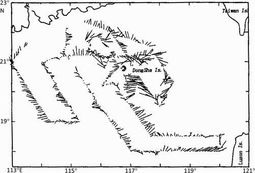
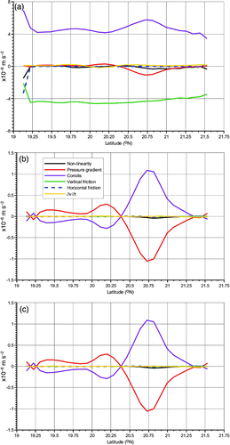
Fig. 10 The variation with latitude of the magnitudes of all terms in the y-direction momentum equation along the 120°50′E longitudinal section at (a) the surface, (b) 100 m and (c) 200 m depths.

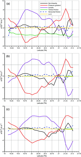
Fig. 11 The variation with latitude of K1, K2, K3 and K4 along the 120°50′E longitudinal section at (a) the surface, (b) 100 m and (c) 200 m depths.

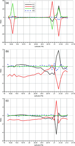
Fig. 12 As in Fig. 10 except for 120°40′E.

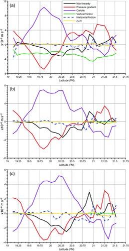
Fig. 13 As in Fig. 10 except for 121°00′E.

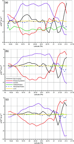
Fig. 14 As in Fig. 10 except for Case 2 with the homogeneous density field.

Xu , J. P. and Su , J. L. 1997 . Hydrographic analysis on the intrusion of Kuroshio into the South China Sea-II. Observational results during the cruise from August to September in 1994 . Tropic Oceanology , 16 ( 2 ) : 1 – 23 . (in Chinese with English abstract)

 Google Scholar