629
Views
1
CrossRef citations to date
0
Altmetric
Fundamental Research / Recherche fondamentale

Improving Statistical Downscaling of General Circulation Models

, , &
Pages 213-225 | Received 03 Apr 2012, Accepted 26 Nov 2012, Published online: 12 Mar 2013

Figures & data

Fig. 1 Grid boxes from a general circulation model (CGCM3) with horizontal resolution of about 300 km by 400 km are plotted over Atlantic Canada. Observations used in this study were taken at Shearwater Airport, Nova Scotia, Canada (44.63°N, 63.5°W). Shearwater Airport (red dot) is about 4 km east of the downtown core of Halifax, Nova Scotia, Canada.
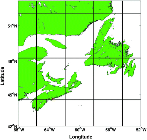
Fig. 1 Grid boxes from a general circulation model (CGCM3) with horizontal resolution of about 300 km by 400 km are plotted over Atlantic Canada. Observations used in this study were taken at Shearwater Airport, Nova Scotia, Canada (44.63°N, 63.5°W). Shearwater Airport (red dot) is about 4 km east of the downtown core of Halifax, Nova Scotia, Canada.

Fig. 2 The black line in (a) represents observed T min (degrees Celsius) from Shearwater Airport, Nova Scotia, for a 5-year period, 1961–65. The red line in (a) represents the fitted seasonal cycle (fitted over the historical period 1961–2000). Time series in (b) represents the daily anomaly constructed by subtracting the red line from the black line in (a). Time series in (c) and (d) are analogous to (a) and (b) except they are for T max.
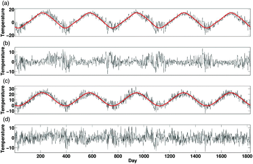
Fig. 2 The black line in (a) represents observed T min (degrees Celsius) from Shearwater Airport, Nova Scotia, for a 5-year period, 1961–65. The red line in (a) represents the fitted seasonal cycle (fitted over the historical period 1961–2000). Time series in (b) represents the daily anomaly constructed by subtracting the red line from the black line in (a). Time series in (c) and (d) are analogous to (a) and (b) except they are for T max.

Table 1. Regression coefficients for the seasonal cycles of observed T min and T max at Shearwater, Nova Scotia, in units of degrees Celsius.

Table 2. Original names (set of 25) of NCEP and CGCM3 predictors. The subsets for each season chosen through the predictor selection process are also shown by the checkmark. Winds in the table are geostrophic winds.

Fig. 3 (a) Time series of the geopotential height (blue) at 500 hPa produced by the CGCM3 at the model grid box containing Shearwater, Nova Scotia, during the period 2001–70. The vertical red dotted lines divide the future period into three separate future periods: 2001–10, 2011–40 and 2041–70. The black line in (a) represents the linear trend (with the mean) in each future period. The seasonal cycle fitted to each future period (red, green, magenta) detrended data (geopotential height (blue) minus trend (black)) is also shown in (a). Time series in (b) are daily anomalies constructed by taking the geopotential height minus the trend in each period and finally subtracting the seasonal cycle in each future period. Panel (b) also shows the seasonal cycle mean which was added for each period as the final step.
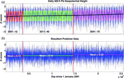
Fig. 3 (a) Time series of the geopotential height (blue) at 500 hPa produced by the CGCM3 at the model grid box containing Shearwater, Nova Scotia, during the period 2001–70. The vertical red dotted lines divide the future period into three separate future periods: 2001–10, 2011–40 and 2041–70. The black line in (a) represents the linear trend (with the mean) in each future period. The seasonal cycle fitted to each future period (red, green, magenta) detrended data (geopotential height (blue) minus trend (black)) is also shown in (a). Time series in (b) are daily anomalies constructed by taking the geopotential height minus the trend in each period and finally subtracting the seasonal cycle in each future period. Panel (b) also shows the seasonal cycle mean which was added for each period as the final step.

Fig. 4 Distributions of T mean in (a) winter and (b) summer generated from NCEP (black) and CGCM3 (red) datasets between 1961 and 2000 at Shearwater, Nova Scotia. Both the NCEP and CGCM3 predictors are Z-scores. The distribution is created by binning the data in bins 0.5 of a Z-score wide. The probability is calculated by taking the number of measurements occurring in each bin and dividing by the total number of measurements.
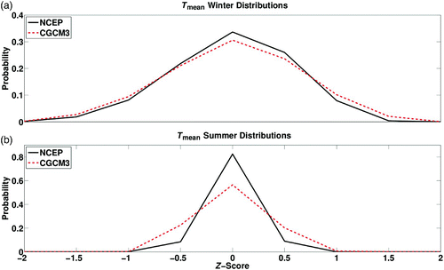
Fig. 4 Distributions of T mean in (a) winter and (b) summer generated from NCEP (black) and CGCM3 (red) datasets between 1961 and 2000 at Shearwater, Nova Scotia. Both the NCEP and CGCM3 predictors are Z-scores. The distribution is created by binning the data in bins 0.5 of a Z-score wide. The probability is calculated by taking the number of measurements occurring in each bin and dividing by the total number of measurements.

Table 3. The numbers in the percent (%) column refer to the fraction of total variance explained in the original dataset by each of the seventeen principal components (PCs) for winter. Here R refers to the correlation coefficient of each PC with T min and T max, and γ refers to the regression coefficient, in units of degrees Celsius, of those PCs used in the winter regression.

Table 4. The numbers in the percent (%) column refer to the fraction of total variance explained in the original dataset by each of the fifteen Principal Components (PCs) for summer. Here R refers to the correlation coefficient of each PC with T min and T max, and γ refers to the regression coefficient, in units of degrees Celsius, of those PCs used in the summer regression.

Table 5. The percentage of total variance explained by the regression for T min and T max during the training period (1961–90) and the validation period (1991–2000) for winter and summer.

Fig. 5 (a) Time series of observed daily anomalies of T min (degrees Celsius) in winter (black) for two years (1990–91). The NCEP prediction of the daily T min anomaly in winter for the last year of the training period (1990) is shown in red. The blue line represents the winter T min NCEP prediction of the daily anomaly for the first year of the validation period (1991). (b) As in (a) except for T max in winter. Time series in (c) and (d) are the same as in (a) and (b), except for summer.
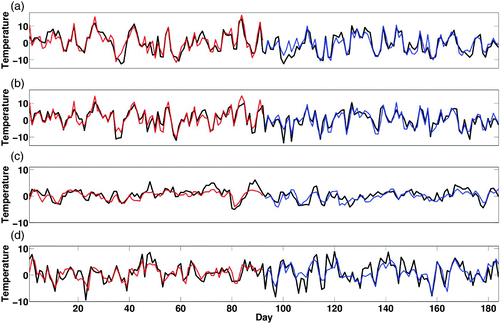
Fig. 5 (a) Time series of observed daily anomalies of T min (degrees Celsius) in winter (black) for two years (1990–91). The NCEP prediction of the daily T min anomaly in winter for the last year of the training period (1990) is shown in red. The blue line represents the winter T min NCEP prediction of the daily anomaly for the first year of the validation period (1991). (b) As in (a) except for T max in winter. Time series in (c) and (d) are the same as in (a) and (b), except for summer.

Fig. 6 Distributions of the observed (black), CGCM3 predicted (red dashed) and raw CGCM3 (blue dashed) total T min and T max in winter and summer for the period 1961–2000. To create the distribution the data were separated into bins that were two degrees Celsius wide over the range of the data. The sample probability on the vertical axis refers to the number of measurements occurring within a particular bin divided by the total number of measurements.
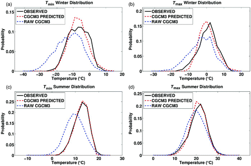
Fig. 6 Distributions of the observed (black), CGCM3 predicted (red dashed) and raw CGCM3 (blue dashed) total T min and T max in winter and summer for the period 1961–2000. To create the distribution the data were separated into bins that were two degrees Celsius wide over the range of the data. The sample probability on the vertical axis refers to the number of measurements occurring within a particular bin divided by the total number of measurements.

Fig. 7 Distribution of CGCM3 predicted total T max and T min in winter and summer in the historical period (1961–90) and three future periods (2011–40, 2041–70, 2071–2100). The distributions are created by binning the data in two degree Celsius bins. The sample probability is found by dividing the number of measurements in a particular bin by the total number of measurements.
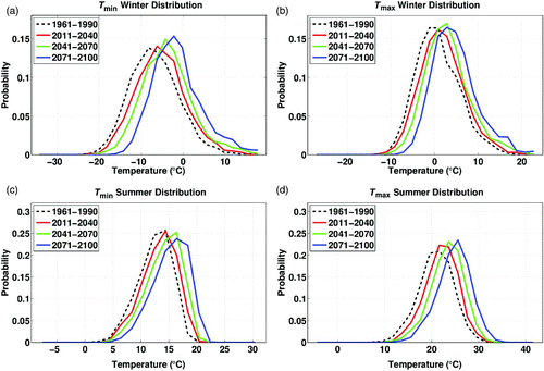
Fig. 7 Distribution of CGCM3 predicted total T max and T min in winter and summer in the historical period (1961–90) and three future periods (2011–40, 2041–70, 2071–2100). The distributions are created by binning the data in two degree Celsius bins. The sample probability is found by dividing the number of measurements in a particular bin by the total number of measurements.

Table 6. The mean and standard deviation for the predicted future distributions of CGCM3-predicted total T min in the winter and summer seasons for the three future periods (2011–40, 2041–70, 2071–2100). The change in mean (δμ ) from the historical to each future tri-decade is also shown. The historical observed distribution mean and standard deviation are also shown. The units in this table are degrees Celsius.

Table 7. The mean and standard deviation for the predicted future distributions of CGCM3-predicted total T max in the winter and summer seasons for the three future periods (2011–40, 2041–2070, 2071–2100). The change in mean (δμ ) from the historical to each future tri-decade is also shown. The historical observed distribution mean and standard deviation are also shown. The units in this table are degrees Celsius.

Table 8. Values of γ 2 for predicting the daily anomalies of T min and T max in winter and summer during the historical period (1961–2000) using the SD method with and without removal of the seasonal cycles from predictors and predictands prior to training the regression model. Values of γ 2 in predicting T max with SDSM are also shown.

Reprints and Corporate Permissions

Please note: Selecting permissions does not provide access to the full text of the article, please see our help page How do I view content?

To request a reprint or corporate permissions for this article, please click on the relevant link below:

Academic Permissions

Please note: Selecting permissions does not provide access to the full text of the article, please see our help page How do I view content?

Obtain permissions instantly via Rightslink by clicking on the button below:

If you are unable to obtain permissions via Rightslink, please complete and submit this Permissions form. For more information, please visit our Permissions help page.