Figures & data
Fig. 1 Map of the LFV showing selected Metro Vancouver monitoring station locations (numbered triangles), urban areas of note (red), and important bodies of water and local elevation (shading).
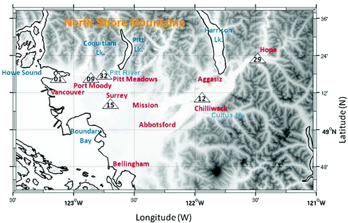
Fig. 2 Time series plots of the 3-year running average of the fourth highest 8-hour averaged ozone concentration (open circles) at T09 (Port Moody), T15 (Surrey East), T12 (Chilliwack) and T29 (Hope). The green line in each plot is the CWS of 65 ppb. Trend lines are also included. Red lines indicate statistically significant (95% level) trends whereas blue lines are not statistically significant.
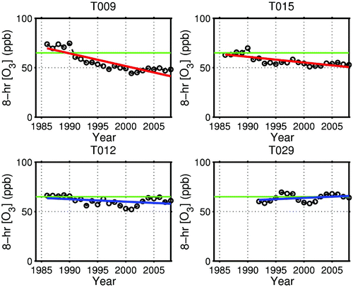
Table 1. List of model simulations showing simulation purpose, type of meteorology used, emissions inventory year and levels, other simulation details as well as the figure number where the simulation results are presented. For a breakdown of annual emission rates by emission sector, please refer to the document prepared by Metro Vancouver (Citation2007).
Fig. 3 The modelled percentage change in ozone concentration (dO3) to a percentage change in emissions (dE) of either VOC (blue crosses) or NOx (purple circles) as a function of the modelled ratio of [O3]/[NOy].
![Fig. 3 The modelled percentage change in ozone concentration (dO3) to a percentage change in emissions (dE) of either VOC (blue crosses) or NOx (purple circles) as a function of the modelled ratio of [O3]/[NOy].](/cms/asset/aaa89975-863e-41a2-bb21-42a25c1bb836/tato_a_782264_o_f0003g.jpg)
Fig. 4 Modelled maximum 8-hour average ozone exposure field (in ppb) over day 1 using Type I meteorology (24 June 2006) for (a) 1985 emissions and (b) 2005 emissions. Also shown is the predicted VOC/NOx ridgeline based on the [O3]/[NOy] ratio (magenta) and the fixed monitoring network station locations (black squares).
![Fig. 4 Modelled maximum 8-hour average ozone exposure field (in ppb) over day 1 using Type I meteorology (24 June 2006) for (a) 1985 emissions and (b) 2005 emissions. Also shown is the predicted VOC/NOx ridgeline based on the [O3]/[NOy] ratio (magenta) and the fixed monitoring network station locations (black squares).](/cms/asset/08208387-d42c-4521-a454-010f69f6a67e/tato_a_782264_o_f0004g.jpg)
Fig. 5 As in but valid for day 2 using Type II meteorology (11 August 2001).
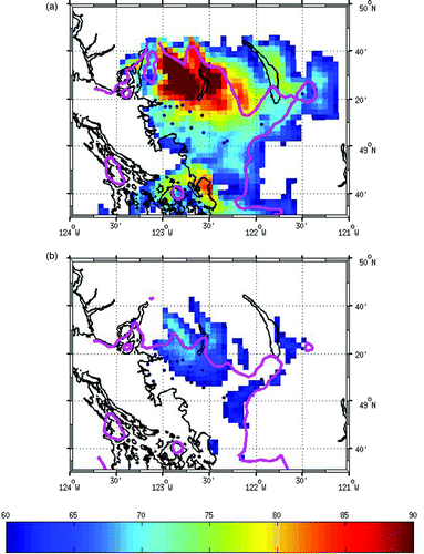
Fig. 6 As in but valid for day 2 using Type III meteorology (18 July 1995).
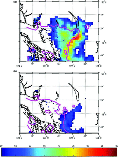
Fig. 7 As in but valid for day 2 using Type IV meteorology (20 July 1985).
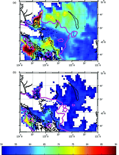
Fig. 8 The predicted VOC/NOx ridgeline based on the [O3]/[NOy] = 7 ratio for all twelve modelled days (four episodes of three days each) using 1985 emissions (red dots) and for all days using 2005 emissions (blue dots). The solid red (blue) line gives the approximate mean position of the 1985 (2005) ridgeline. Also shown are the fixed monitoring network station locations (black squares). For clarity, the ridgelines were truncated west of Vancouver. The coloured areas show the percentage difference in the LFV population density between 2005 and 1985. The blue areas show grid cells whose population density (percentage of total LFV residing in that grid cell) have declined, and the red areas show grid cells whose percentage of the total LFV population have increased.
![Fig. 8 The predicted VOC/NOx ridgeline based on the [O3]/[NOy] = 7 ratio for all twelve modelled days (four episodes of three days each) using 1985 emissions (red dots) and for all days using 2005 emissions (blue dots). The solid red (blue) line gives the approximate mean position of the 1985 (2005) ridgeline. Also shown are the fixed monitoring network station locations (black squares). For clarity, the ridgelines were truncated west of Vancouver. The coloured areas show the percentage difference in the LFV population density between 2005 and 1985. The blue areas show grid cells whose population density (percentage of total LFV residing in that grid cell) have declined, and the red areas show grid cells whose percentage of the total LFV population have increased.](/cms/asset/99ae353e-bd10-4476-9cc2-32d8e40ebe84/tato_a_782264_o_f0008g.jpg)
Fig. 9 Spatial plot of the average decrease (in ppb) between 1985 and 2005 in the modelled 8-hour averaged ozone exposure. The 8-hour exposure field was averaged over each of the three days in each of the four exploration runs. Also shown are the monitoring network station locations (green triangles) and contours at 8, 12, and 16 ppb (thin black lines).
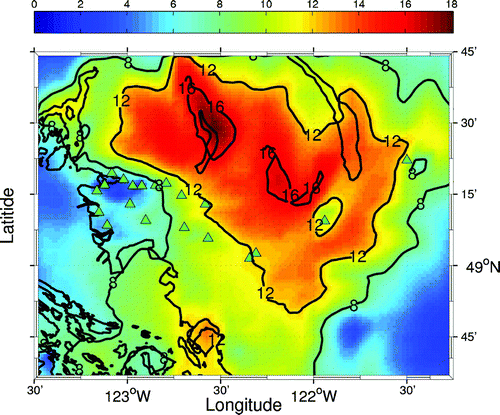
Fig. 10 Time series plots of the modelled difference in the average diurnal ozone concentrations (ppb) at T01, T09, T12, and T29 between runs with 1985 emissions/1985 spatial surrogates and 2005 emissions/2005 spatial surrogates (red curves); 1985 emissions/2005 spatial surrogates and 2005 emissions/2005 spatial surrogates (blue curves); 2005 emissions/1985 spatial surrogates and 2005 emissions/2005 spatial surrogates (green curves). Positive values for the blue curve represent lower ozone concentrations arising from 1985 to 2005 emissions reductions only; positive values for the green curve represent lower ozone concentrations arising from 1985 to 2005 population density changes only; and positive values for the red curve represent lower ozone concentrations arising from a combination of lower emissions and changing (1985 to 2005) population densities.
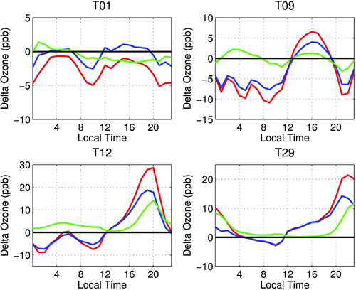
Fig. 11 Ozone isopleth schematic showing ozone response surface (blue lines) as a function of VOC and NOx concentrations. The green line represents the ridgeline. Also shown is the time series of yearly mean 8-hour average summertime VOC (red) and NOx (blue) concentrations (restricted to days with VOC measurements) observed at T09 (upper left), T12 (upper right), and T29 (lower left). The bottom right plot shows time series plots of scaled VOC (red) and NOx (blue) emissions over the LFV. Each curve has been scaled so that its value in 1985 is equal to 100. Overlaid on the isopleth diagram is an estimate of how the ozone response to precursor emissions at T09, T12, and T29 has changed over the 1985–2005 period (dashed red lines).
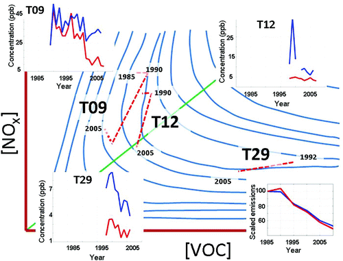
Fig. 12 Average diurnal ozone concentration profile at Port Moody (T09: circles) and Chilliwack (T12: squares) from the 1985–90 (red) and 2000–05 (blue) periods. Each curve has been normalized to highlight the temporal evolution of the diurnal profile better.
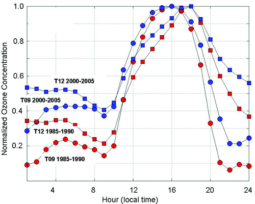
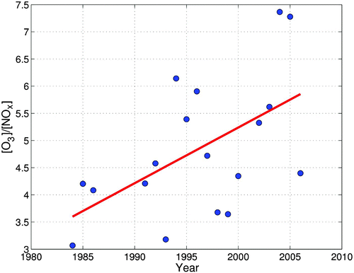
Fig. 13 Ratio of 8-hour average ozone to 8-hour average NOx concentrations between 1984 and 2006 (blue dots) at T12 along with the trend line (red line). Yearly values are based on 8-hour averages of the seven days with the highest hourly ozone concentrations.