Stratospheric Polar Vortex Splitting in December 2009

Figures & data

Fig. 1 Evolution of daily zonal mean temperature (K) at 70 hPa averaged over 80°–90°N for December 2009 to April 2010 (red), 2010 to 2011 (blue), and the climatological means for the period 1968 to 1996 (green).

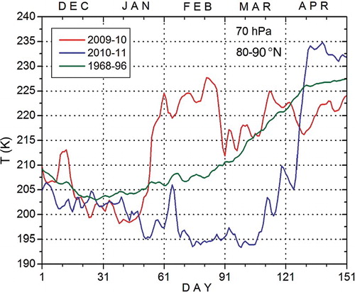
Fig. 2 Evolution of the daily zonal mean temperature (K) at 70 hPa averaged over 80°–90°N (blue, right axis), the mean zonal wind (m s⁻¹) at 10 hPa averaged over 60°–70°N (green), and the zonal meridional heat flux (K m s⁻¹) at 100 hPa averaged over 50°–70°N (magenta) from December 2009 to March 2010 (left axis).

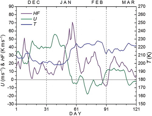
Fig. 3 Evolution of the daily amplitudes of the planetary waves with wavenumber k = 1, 2, and 3 (blue, red, and green lines, respectively), in geopotential height (m) averaged over the latitudinal band 40°–75°N at (a) 30 hPa and (b) 300 hPa from 1 December 2009 to 30 April 2010.

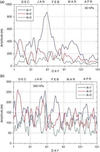
Fig. 4 Stereographic projections of potential vorticity (10⁻⁵ K m² kg⁻¹ s⁻¹) at isentropic level 530 K (approximately 30 hPa) on (a) 7 December, (b) 10 December, (c) 14 December, and (d) 18 December 2009. The contour interval is 1×10⁻⁵ K m² kg⁻¹ s⁻¹; shading indicates potential vorticity larger than 4×10⁻⁵ K m² kg⁻¹ s⁻¹. The southern edge of the projection is 12°N.

Fig. 5 Time-longitude diagram of daily squared meridional velocity (m² s⁻²) averaged over (a) 30°–50°N and (b) 70°–80°N at 200 hPa from 26 November to 31 December 2009. The red arrows indicate the direction of the group velocity of the Rossby wave train before the vortex splits. Contours are 200, 300, 400, 500, 600 m² s⁻² and at 300 m² s⁻² intervals thereafter.

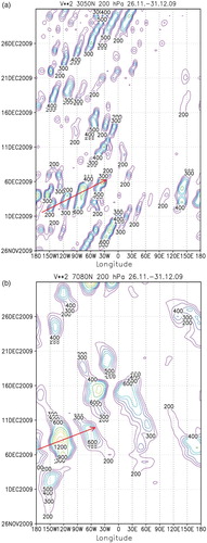
Fig. 6 Latitude-longitude cross-sections of negative OLR anomalies (W m⁻²) from the corresponding climatological mean averaged over (a) 26 to 28 November and (b) 29 November to 1 December.

Fig. 7 Stereographic projections of horizontal components (F_x, F_y) of Plumb fluxes (m² s⁻²) (indicated by arrows) and the deviation of geopotential height G* (m) (contours, interval 100) from zonal mean at 300 hPa averaged over (a) 1–3, (b) 3–5, (c) 5–7, and (d) 7–9 December 2013. The southern edge of the projection is 20°N. The scale of the fluxes is indicated by the arrow below each plot (m² s⁻²).

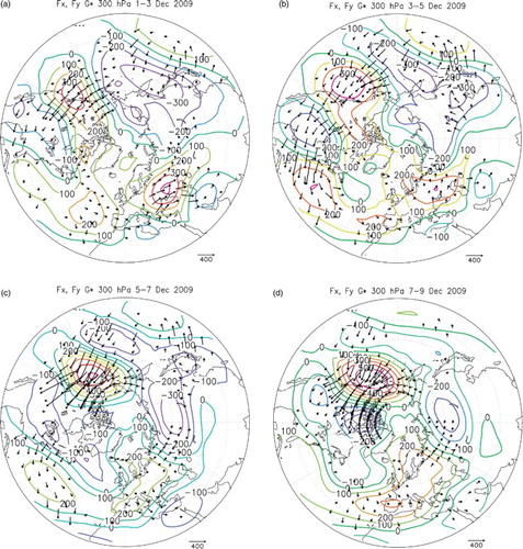
Fig. 8 Height-longitude cross-sections of the vertical and longitudinal components (F_x, F_z) of the Plumb fluxes (m² s⁻²) and the deviation of geopotential height G* from the zonal mean (m) averaged over the latitudinal band 30°–50°N (left column) and 50°–70°N (right column) on 3–5 December (a) and (b), 5–7 December (c) and (d), and 7–9 December (e) and (f) 2009. The vertical component of wave activity flux is multiplied by a factor of 100. The scale of the fluxes is indicated by the arrow below each plot (m² s⁻²).

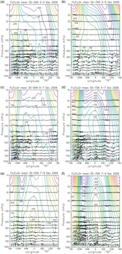
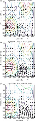
Fig. 9 Height-latitude cross-sections of the vertical and latitudinal components (F_y, F_z) of the mean zonal Plumb fluxes (m² s⁻²) and mean zonal wind U (ms⁻¹) on (a) 3–5 December, (b) 5–7 December, and (c) 7–9 December 2009. The scale of the fluxes is indicated by the arrow below each plot (m² s⁻²).