Figures & data
Fig. 1 Schematic illustrating spatial fringes created from wavefronts in the SHS. The figure is reproduced from Harlander et al. (Citation1992) by permission of the AAS.
Fig. 2 Schematic layout for the Doppler Asymmetric Spatial Heterodyne Spectrometer (DASH; reproduced from Englert et al. (Citation2007)).
Fig. 3 SWIFT-DASH monolithic optics assembly. The reddish elements are the ZnSe optical components. The clear BSL7 glass spacers are hollowed out in the optical path. The optics as shown are 540 mm wide, 260 mm deep, and 100 mm high.
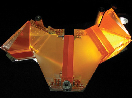
Fig. 4 SWIFT-DASH monolithic optics assembled in a rigid frame. The gratings are visible in each arm.
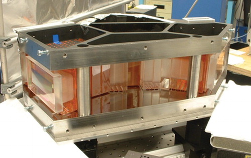
Fig. 5 Raw image of fringes observed following final assembly of the SWIFT-DASH monolithic optics. The observations were made at room temperature and in air with a FLIR SC7300 L IR camera (320 pixels × 256 pixels).
Fig. 6 Radiance spectra from the atmospheric radiative transfer model (RTS) developed for SWIFT. Spectra are simulated line by line at various tangent altitudes. Two isotopic N2O lines and one NH3 line are shown; these provide reference calibration lines.
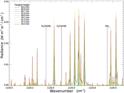
Fig. 7 Altitude profiles of simulated amplitudes (given in Analogue to Digital Units (ADU) assuming a 14 bit Analogue to Digital Converter (ADC)) for selected fringe frequencies used in the retrievals.
Fig. 8 Retrieved ozone (red) profile compared with a simulated mid-latitude summer “true” profile (blue). The first guess profile is shown in green.
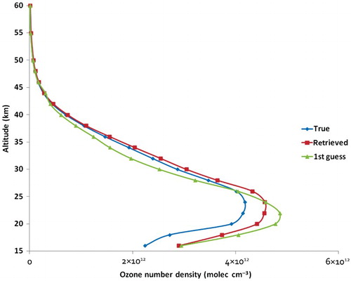
Fig. 9 Error in the retrieved ozone profile (percentage relative to “true”).
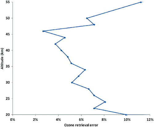
Fig. 10 Retrieved wind profile (red) compared with simulated “true” (blue) profile. The first guess profile is shown in green.
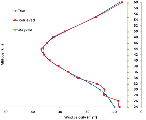
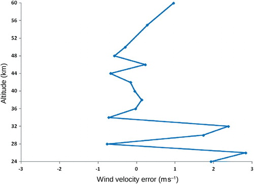
Fig. 11 Error in the retrieved wind profile (relative to “true”).