Statistical Projections of Ocean Climate Indices off Newfoundland and Labrador

Figures & data

Fig. 1 Map showing the study region. Station 27 (red diamond), the Flemish Cap transect (black line), and the area with the fall bottom temperature data (dashed lines) are indicated.

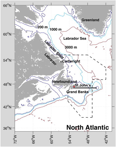
Table 1. Means and standard deviations for the 1981–2010 reference period (SST: sea surface temperature; CIL: cold intermediate layer; BT: bottom temperature). See Fig 1 for locations.

Variable	1981–2010 Mean	Standard Deviation
SST (°C) at Station 27	5.18	0.82
CIL (km^2) at the Flemish Cap transect	26.52	6.63
Fall BT (°C) over the Newfoundland and Labrador Shelves	1.61	0.50
Winter SIE (10^5 km^2)	1.96	0.81
Number of icebergs at 48°N	813	648
NAO (hPa)	20.44	8.77
St. John's air temperature (°C)	5.03	0.84
Cartwright air temperature (°C)	0.05	1.32

Fig. 2 Scatter diagram between the observed sea surface temperature anomalies (SST, °C) at Station 27 and the observed air temperature anomalies (°C) at St. John's from 1950 to 2010. The lines show the linear fits to the annual-mean observations.

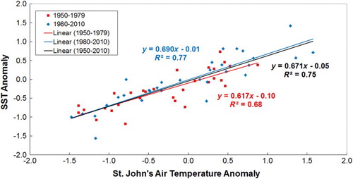
Fig. 3 Reconstructed SST anomalies (°C) at Station 27 based on simulated air temperature anomalies at St. John's. The air temperatures are the CanESM2 and GFDL-ESM2M output under RCP4.5 and RCP8.5 and the CRCM output under A1B. The straight lines are the linear fits to the SST projections for 2011–2100 or 2011–2070.

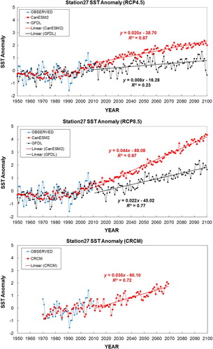
Table 2. Linear trends and associated standard errors.

		A1B	RCP4.5	RCP8.5
	1970–2010
SST (°C y^−1)	Observed	0.023 ± 0.008
	CanESM2	–	0.021 ± 0.003	0.022 ± 0.003
	GFDL-ESM2M	–	0.012 ± 0.005	0.018 ± 0.005
	CRCM	0.019 ± 0.004	–	–
	1978–2010
BT (°C y^−1)	Observed	0.049 ± 0.013
	CanESM2	–	0.034 ± 0.004	0.034 ± 0.004
	GFDL-ESM2M	–	0.012 ± 0.006	0.020 ± 0.006
	CRCM	0.018 ± 0.006	–	–
	1970–2011
CIL (km^2 y^−1)	Observed	−0.211 ± 0.083
	CanESM2	–	−0.178 ± 0.020	−0.191 ± 0.022
	GFDL-ESM2M	–	−0.078 ± 0.033	0.094 ± 0.033
	CRCM	−0.131 ± 0.047	–	–
	1970–2011
SIE (10^5 km^2 y^−1)	Observed	−0.031 ± 0.009
	CanESM2	–	−0.028 ± 0.003	−0.030 ± 0.003
	GFDL-ESM2M	–	−0.012 ± 0.005	−0.015 ± 0.005
	CRCM	−0.020 ± 0.007	–	–
	1983–2011
Icebergs (y^−1)	Observed	−31 ± 14
	CanESM2	–	−25 ± 3	−26 ± 2
	GFDL-ESM2M	–	−9 ± 4	−15 ± 4
	CRCM	−13 ± 4	–	–

Fig. 4 Scatter diagram between the observed fall bottom temperature anomalies (BT, °C) over the Newfoundland and Labrador Shelves and the observed air temperature anomalies (°C) at Cartwright from 1978 to 2010. The line is the linear fit to the observations.

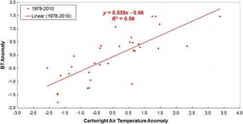
Fig. 5 Reconstructed fall bottom temperature anomalies (BT, °C) over the Newfoundland and Labrador Shelves based on simulated air temperature anomalies at Cartwright. The air temperatures are the CanESM2 and GFDL-ESM2M output under RCP4.5 and RCP8.5 and the CRCM output under A1B. The straight lines are the linear fits to the BT projections for 2011–2100 or 2011–2070.

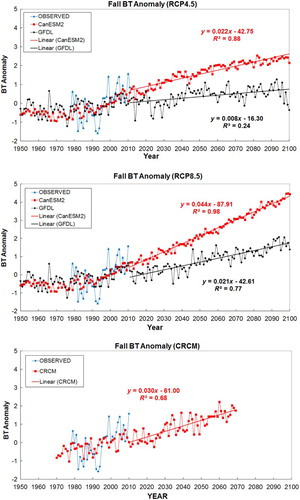
Fig. 6 Scatter diagram between the observed CIL area anomalies (km²) at the Flemish Cap section and the observed winter air temperature anomalies (°C) at Cartwright from 1951 to 2011. The line is the linear fit to observations.

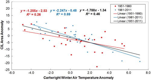
Fig. 7 Reconstructed cold intermediate layer (CIL) area anomalies (km²) along the Flemish Cap transect based on simulated winter air temperature anomalies at Cartwright. The air temperatures are the CanESM2 and GFDL-ESM2M output under RCP4.5 and RCP8.5 and the CRCM output under A1B. The straight lines are linear fits to the CIL projections for 2011–2100 or 2011–2070.

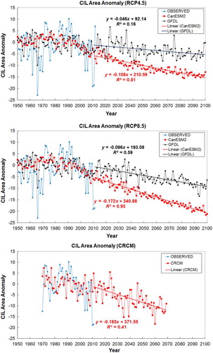
Fig. 8 Scatter diagram between the observed sea-ice extent (SIE) anomalies (×10⁵ km²) off Newfoundland and Labrador and the observed winter air temperature anomalies (°C) at Cartwright from 1963 to 2011. The line is the linear fit to observations

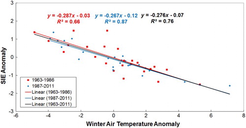
Fig. 9 Reconstructed sea-ice extent anomalies (SIE) (×10⁵ km²) off Newfoundland and Labrador based on the simulated winter air temperature anomalies at Cartwright. The air temperatures are the CanESM2 and GFDL-ESM2M output under RCP4.5 and RCP8.5 and the CRCM output under A1B. The straight lines are the linear fits to the SIE projections from 2011 to 2100. Note that years with SIE anomalies below −1.96×10⁵ km² are ice free.

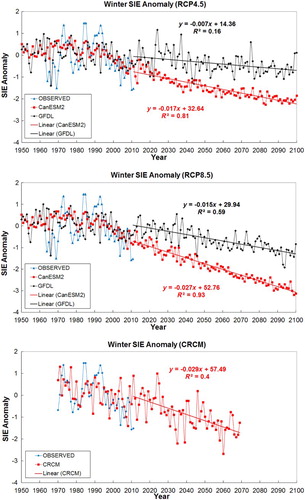
Fig. 10 Scatter diagram between the observed number of iceberg anomalies at 48°N and the observed winter air temperature anomalies (°C) at Cartwright from 1983 to 2011. The line is the linear fit to observations.

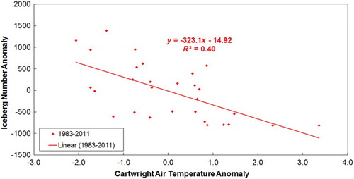
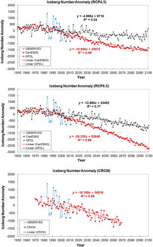
Fig. 11 Reconstructed iceberg number anomalies at 48°N based on simulated winter air temperature anomalies at Cartwright. The air temperatures are the CanESM2 and GFDL-ESM2M output under RCP4.5 and RCP8.5 and the CRCM output under A1B. The straight lines are the linear fits to the projected number of icebergs from 2011 to 2100. Note that years with iceberg number anomalies below −813 are iceberg free.