Explicit Planktic Calcifiers in the University of Victoria Earth System Climate Model, Version 2.9

Figures & data

Fig. 1 UVic ESCM biogeochemical model schematic. Arrows indicate the flux direction of nutrients.

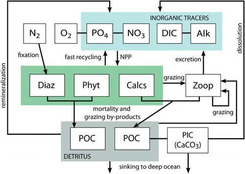
Table 1. Miscellaneous UVic ESCM biogeochemical model parameters. Temperature-dependent parameter values are given for 0°C.

Parameter	Symbol	Units	NOCAL	CAL
Diazotroph growth handicap		unitless	0.4	0.4
E-folding temperature		°C	15.65	15.65
Detrital remineralization rate		d^−1	0.055	0.055
Detrital sinking speed at surface		m d^−1	14.0	14.0
Ballast:Total detrital production ratio		unitless	N/A	0.05
Molar organic P:N ratio		unitless	0.0625	0.0625
Molar organic C:N ratio		unitless	6.625	6.625
Molar organic O:N ratio		unitless	10.0	10.0

Table 2. UVic ESCM CaCO₃ export-production parameters.

Parameter	Symbol	Units	NOCAL	CAL
CaCO3:POC production ratio		unitless	0.03	0.04
CaCO3 dissolution half-saturation constant	k	mmol C m^−3	N/A	100
CaCO3 sinking speed		m d^−1	N/A	35
Light attenuation by CaCO3		(m mmol m^−3)^−1	N/A	0.47

Table 3. UVic ESCM biogeochemical model phytoplankton production parameters. Temperature-dependent parameter values are given for 0°C.

Parameter	Symbol	Units	NOCAL	CAL
Maximum growth rate		d^−1	0.6	0.6
			N/A	0.52
Half-saturation constant N		mmol m^−3	0.7	0.7
			N/A	0.4
Half-saturation approximation constant Fe		nmol m^−3	0.1^a	0.1
			N/A	0.06
			0.1	0.12
Initial slope of P-I^b curve		(W m^−2)^−1 d^−1	0.1	0.1
			N/A	0.06
Light attenuation by phytoplankton		(m mmol m^−3)^−1	0.47	0.43
Phytoplankton mortality rate		d^−1	0.03	0.03
			N/A	0.03
			0.015	0.015
Microbial fast recycling		d^−1	0.015	0.015
			N/A	0.015

^aUVic ESCM value is tuned to an iron mask and is not the actual physiological iron limitation. See Keller et al. (2012) for a detailed discussion.

^bP−I is photosynthesis minus irradiance.

Table 4. UVic ESCM biogeochemical model zooplankton parameters. Temperature-dependent parameter values are given for 0°C.

Parameter	Symbol	Units	NOCAL	CAL
Maximum grazing rate		d^−1	0.4	0.4
Maximum grazing rate parameters		unitless	1.066	1.066
		°C^−1	1.0	1.0
Food preferences		unitless	0.30	0.225
			N/A	0.225
			0.30	0.225
			0.10	0.1
			0.30	0.225
Half-saturation constant		mmol m^−3	0.15	0.15
Growth efficiency constant		unitless	0.4	0.4
Assimilation efficiency		unitless	0.7	0.7
Mortality rate		d^−1	0.06	0.06

Table 5. Globally integrated biological properties.

Property	NOCAL	CAL	Independent Estimate
Primary production (Pg C y^−1)	61.82	64.19	44–78^a
Export production at 130 m (Pg C y^−1)	7.77	7.09	5.73^b
POC flux at 2 km (Pg C y^−1)	0.26	0.36	0.43 ± 0.05^b
CaCO3 export at 130 m (Pg C y^−1)	0.94	0.83	1.1 ± 0.3^c
CaCO3 flux at 2 km (Pg C y^−1)	0.55	0.43	0.41 ± 0.05^b
CaCO3 dissolution (Pg C y^−1)	N/A	0.40	0.5 ± 0.2^d
CaCO3 sediment flux (Pg C y^−1)	0.48	0.42	0.21–0.27^e
Total phytoplankton (Pg C)	0.52	0.47	0.5–2.4^f
Phytoplankton calcifiers (Pg C)	N/A	0.15	0.001–0.03^g
Zooplankton (Pg C)	0.55	0.59	0.03–0.67^h

^aLow value from Carr et al. (2006), high value from Jin et al. (2006). Buitenhuis, Hashioka, and Le Quéré (2013b) recently used a model–data synthesis to constrain the value to 56 Pg C y⁻¹.

^bFrom Honjo et al. (2008).

^cFrom Lee (2001).

^dFrom Feely et al. (2004).

^e0.1–0.14 Pg C y⁻¹ in pelagic zones, 0.11–0.13 Pg C y⁻¹ in coastal zones, from Iglesias-Rodríguez et al. (2002).

^fTotal global autotrophic biomass from Buitenhuis et al. (2013a).

^gFrom Buitenhuis et al. (2013a).

^hCalcifying zooplankton only, from Buitenhuis et al. (2013a).

Fig. 2 Averaged biogeochemical simulated tracers (CAL, solid red line; NOCAL, dashed blue line) compared with observations (black line). DIC and alkalinity observations are the standard GLODAP product (Key et al., 2004). Phosphate and nitrate observations are annual averages from the World Ocean Atlas (WOA; Garcia et al., 2009). Bottom row shows globally averaged model-data misfits.

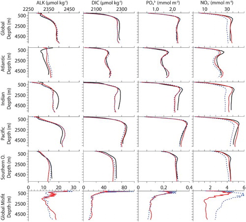
Fig. 3 Normalized Taylor diagrams of simulated tracers (CAL, red symbols; NOCAL, blue symbols) compared with observations (black circle). Observations used are as in Fig. 2. Ocean basins are denoted as global average (star), Atlantic (square), Indian (triangle), Pacific (plus), and Southern Ocean (diamond). The distance to the origin represents the normalized standard deviation. Normalized correlation with the observations is read from the azimuthal position. Perfect agreement with observations is a normalized standard deviation of 1 and a normalized correlation of 1.

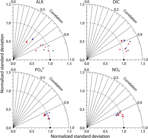
Fig. 4 Depth-integrated annual average PFT biomass (g C m⁻²): (a) CAL general phytoplankton; (b) CAL phytoplankton calcifiers; (c) CAL diazotrophs; (d) CAL zooplankton; (e) NOCAL general phytoplankton; (f) NOCAL diazotrophs; (g) NOCAL zooplankton. Also shown is depth-integrated NPP (g C m⁻² d⁻¹) for (h) CAL and (i) NOCAL.

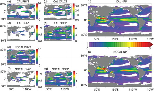
Fig. 5 Zonally averaged by ocean basin and surface distributions (CAL, left column; WOA observations, right column).

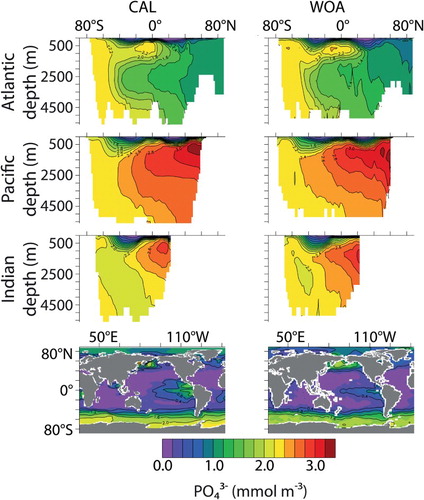
Fig. 6 Zonally averaged DIC by ocean basin and surface distributions (CAL, left column; GLODAP observations, right column).

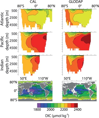
Fig. 7 Zonally averaged alkalinity by ocean basin and surface distributions (CAL, left column; GLODAP observations, right column).

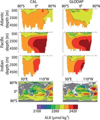
Fig. 8 Zonally averaged CaCO₃ concentration by ocean basin (left and middle panels). Model CAL CaCO₃ concentration, including living CaCO₃ attached to phytoplankton calcifiers and zooplankton, in the surface grid box (to 50 m depth, top right panel). Bottom right is the standard CaCO₃ product from Aqua MODIS, accumulated over the entire mission (2002–2013; NASA, 2013).

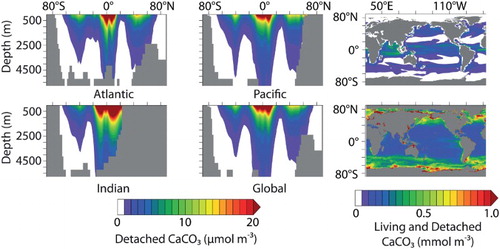
Fig. 9 Regression between modelled and observed CAL CaCO₃ concentration (left panel) and CAL POC concentration (right panel) from the ocean surface to 1000 m depth. Data are in situ measurements from Lam et al. (2011).

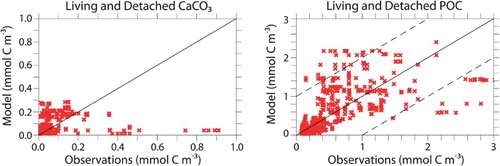
Fig. 10 Normalized Taylor diagram of model CaCO₃ concentrations compared with the Lam et al. (2011) dataset (black circle). Models are CAL (red circle), GFDL-ES2M (green star), MIROC-ESM (light blue circle), CNRM-CM5 (blue diamond), MPI-ESM-LR (yellow plus), and IPSL-CM5B-LR (purple circle). With the exception of CAL, the data for all models were obtained by mining the CMIP5 database (http://cmip-pcmdi.llnl.gov) using the following search terms: CMIP5/ocean biogeochem/pre-industrial control/annual output/calcite concentration.

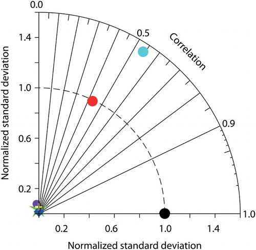
Fig. 11 Model average CaCO₃ (upper left panel) and POC (upper middle panel) export and average POC:CaCO₃ rain ratio (upper right panel) at 2 m depth overlaid by trap data from Honjo et al. (2008). Regressions between modelled and observed values can be seen in bottom panels.

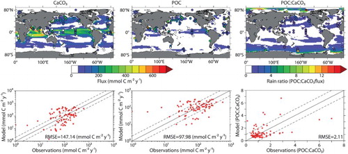
Fig. 12 Percentage CaCO₃ sediment composition. CAL is shown in upper left panel; NOCAL is shown in bottom left panel, and gridded sample data from Archer (1996a) is shown in top right panel.

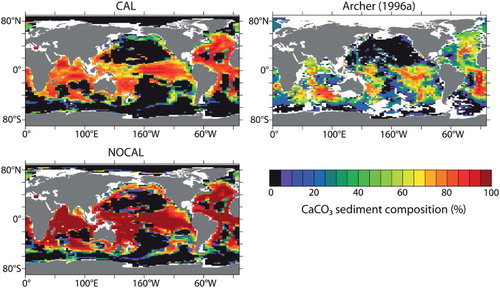
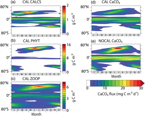
Fig. 13 Hovmöller diagrams of CAL depth-integrated PFT concentrations by latitude and month: (a) phytoplankton calcifiers, (b) general phytoplankton, (c) zooplankton. Also shown is CaCO₃ flux at 130 m depth by latitude and month for (d) CAL and (e) NOCAL.

Keller, D. P., Oschlies, A., & Eby, M. (2012). A new marine ecosystem model for the University of Victoria Earth System Climate Model. Geoscientific Model Development, 5(5), 1195–1220. doi: 10.5194/gmd-5-1195-2012

 Web of Science ®Google Scholar

Carr, M.-E., Friedrichs, M. A. M., Schmeltz, M., Aita, M. N., Antoine, D., Arrigo, K. R., … Yamanaka, Y. (2006). A comparison of global estimates of marine primary production from ocean color. Deep-Sea Research Part II: Topical Studies in Oceanography, 53(5–7), 741–770. doi: 10.1016/j.dsr2.2006.01.028

 Web of Science ®Google Scholar

Jin, X., Gruber, N., Dunne, J. P., Sarmiento, J. L., & Armstrong, R. A. (2006). Diagnosing the contribution of phytoplankton functional groups to the production and export of particulate organic carbon, CaCO3, and opal from global nutrient and alkalinity distributions. Global Biogeochemical Cycles, 20(2). GB2015. doi:10.1029/2005GB002532

 Google Scholar

Buitenhuis, E. T., Hashioka, T., & Le Quéré, C. (2013b). Combined constraints on global ocean primary production using observations and models. Global Biogeochemical Cycles, 27(3), 847–858. doi: 10.1002/gbc.20074

 Web of Science ®Google Scholar

Honjo, S., Manganini, S. J., Krishfield, R. A., & Francois, R. (2008). Particulate organic carbon fluxes to the ocean interior and factors controlling the biological pump: A synthesis of global sediment trap programs since 1983. Progress in Oceanography, 76(3), 217–285. doi: 10.1016/j.pocean.2007.11.003

 Web of Science ®Google Scholar

Lee, K. (2001). Global net community production estimated from the annual cycle of surface water total dissolved inorganic carbon. Limnology and Oceanography, 46(6), 1287–1297. doi: 10.4319/lo.2001.46.6.1287

 Web of Science ®Google Scholar

Feely, R. A., Sabine, C. L., Lee, K., Berelson, W., Kleypays, J., Fabry, V. J., & Millero, F. (2004). Impact of anthropogenic CO2 on the CaCO3 system in the oceans. Science, 305(5682), 362–366. doi: 10.1126/science.1097329

 PubMed Web of Science ®Google Scholar

Iglesias-Rodrlguez, M. D., Armstrong, R., Feely, R., Hood, R., Kleypas, J., Milliman, J. D., … Sarmiento, J. (2002). Progress made in study of ocean's calcium carbonate budget. EOS, Transactions American Geophysical Union, 83(34), 365–375. doi: 10.1029/2002EO000267

 Google Scholar

Buitenhuis, E. T., Vogt, M., Moriarty, R., Bednarsek, N., Doney, S. C., Leblanc, K., … Swan, C. (2013a). MAREDAT: Towards a world atlas of MARine Ecosystem DATa. Earth System Science Data, 5(2), 227–239. doi: 10.5194/essd-5-227-2013

 Google Scholar

Key, R., Kozyr, A., Sabine, C., Lee, K., Wanninkhof, R., Bullister, J., … Mordy, C. (2004). A global ocean carbon climatology: Results from GLODAP. Global Biogeochemical Cycles, 18. doi:10.1029/2004GB002247

 Web of Science ®Google Scholar

Garcia, H. E., Locarnini, R., Boyer, T., Antonov, J., Zweng, M., Baranova, O., & Johnson, D. (2009). World Ocean Atlas 2009: Nutrients (phosphate, nitrate, silicate) (Vol. 4) (No. NOAA Atlas NESDIS 71). Washington, DC: U.S. Government Printing Office.

 Google Scholar

NASA (National Aeronautics and Space Administration). (2013). MODIS PIC data product [Data] (Tech. Rep.). Greenbelt, MD, USA: Goddard Space Flight Center, Distributed Active Archive Center. Retrieved from http://oceancolor.gsfc.nasa.gov/cms/citations

 Google Scholar

Lam, P. J., Doney, S. C., & Bishop, J. K. B. (2011). The dynamic ocean biological pump: Insights from a global compilation of particulate organic carbon, CaCO3, and opal concentration profiles from the mesopelagic. Global Biogeochemical Cycles, 25. doi:10.1029/2010GB003868

 Web of Science ®Google Scholar

Archer, D. (1996a). An atlas of the distribution of calcium carbonate in sediments of the deep sea. Global Biogeochemical Cycles, 10(1), 159–174. doi: 10.1029/95GB03016

 Web of Science ®Google Scholar