Trends and Variability in Sea Ice and Icebergs off the Canadian East Coast

Figures & data

Fig. 1 Map of the northwest Atlantic showing the five sea-ice regions (blue polygons), seven air temperature grid squares (dashed red squares), paleoclimate temperature site (red dot), and communities referred to in the text (green dots); GSL: Gulf of St. Lawrence, Nfld: Newfoundland.

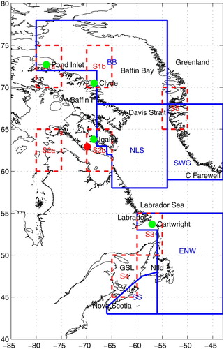
Fig. 2 Ice area or extent anomalies for (left) winter and (right) summer, using1961–1990 as a reference period. Anomalies of ice area for winter (January–March) and summer (June–September) are given for BB and NLS, and of ice extent for winter (February–April) are given for ENW and SS. The anomaly of the ice extent index for summer (May–July) is given for SWG. The blue and red lines show the unsmoothed and 5-year running means, respectively.

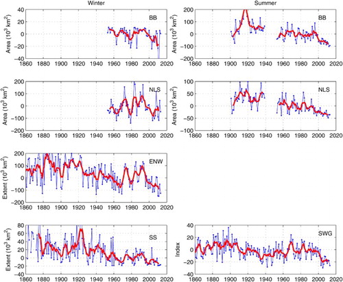
Fig. 3 Ice area anomalies in BB, NLS, and ENW for (left) spring (April–June) and (right) autumn (October–December). The blue and red lines show the unsmoothed and 5-year running means, respectively.

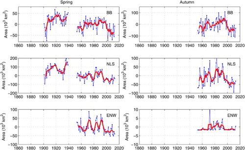
Fig. 4 (top) Annual iceberg season length anomaly, (middle) iceberg flux past 48°N anomaly, and (bottom) number of extreme observations of icebergs (October–September). The blue and red lines show the unsmoothed and 5-year running means, respectively. In the bottom panel, the shaded area represents the recent period not covered by the dataset.

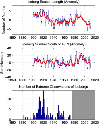
Table 1. Trends (T) in sea-ice area for the BB, NLS, ENW, and SS regions (percent per decade) and iceberg season length south of 48°N, iceberg season length (ISL; months per decade); correlation coefficients (r) of ice area with linear trends are also shown. The three numbers in each cell refer to the periods 1900–2011, 1953–2011, and 1980–2011, respectively. Winter is January–March; Spring is April–June; Summer is July–September; Autumn is October–December. For the ENW and SS regions in winter, ice extent was used instead of ice area and the time period was February–March. Trends and correlation coefficients significant at the 5% level are shown in bold.

		Winter			Spring			Summer			Autumn
		1900–2011	1953–2011	1980–2011	1900–2011	1953–2011	1980–2011	1900–2011	1953–2011	1980–2011	1900–2011	1953–2011	1980–2011
BB	T	–	−0.5	−1.3	−0.6	−0.3	−3.1	−5.5	−6.8	−16.8	–	0.2	−6.4
	r	–	−0.35	−0.43	−0.36	−0.10	−0.53	−0.57	−0.37	−0.51	–	0.02	−0.45
NLS	T	–	0.0	−8.8	−2.9	−2.6	−10.3	−6.5	−11.2	−25.5	–	−2.5	−20.5
	r	–	0.00	−0.43	−0.57	−0.29	−0.60	0.63	−0.51	−0.65	–	−0.11	−0.68
ENW	T	−4.0	−2.9	−16.5	–	−6.2	−19.9	–	–	–	–	1.5	−34.8
	r	−0.43	−0.14	−0.49	–	−0.24	−0.43	–	–	–	–	0.01	−0.51
SS	T	−7.5	−8.0	−21.4	–	–	–	–	–	–	–	–	–
	R	−0.45	−0.20	−0.35	–	–	–	–	–	–	–	–	–
ISL	T	−0.3	−0.1	−1.5
	r	−0.39	−0.07	−0.57

Fig. 5 Seasonal air temperature anomalies from the CRUTEM4 dataset for (left) winter (December–February) and (right) summer (June–August) for grid squares S1–S5 in Fig. 1, with the y-axis inverted. The blue and red lines show the unsmoothed and 5-year running means, respectively. The reconstructed air temperature (5-year running mean) from Upper Soper Lake paleoclimate data is shown in green.

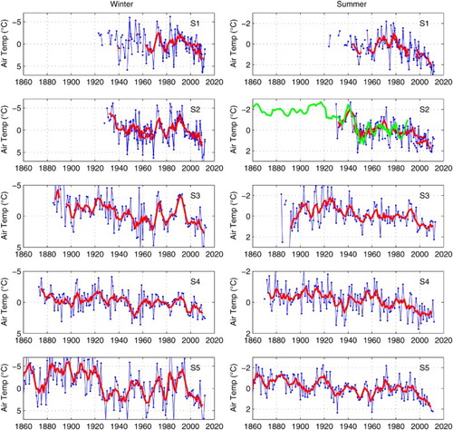
Fig. 6 Seasonal air temperature anomalies from the CRUTEM4 dataset for (left) spring (March–May) and (right) autumn (September–November) for grid squares S1–S5 in Fig. 1, with the y-axis inverted. The blue and red lines show the unsmoothed and 5-year running means, respectively.

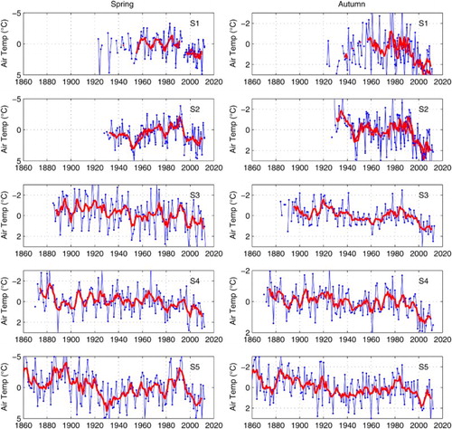
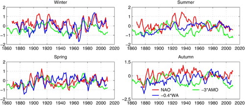
Fig. 7 Seasonal NAO, WA (inverted), and AMO (inverted) anomalies shown as 5-year running means for winter (December-February), spring (March-May), summer (June-August), and autumn (September-November). NAO index data provided by the Climate Analysis Section, National Center for Atmospheric Research, Boulder, Colorado, USA, Hurrell (1995); AMO (Enfield et al., 2001) data, and GPH data from the Twentieth Century Reanalysis (Compo et al., 2011) used to compute WA were provided by the National Oceanographic and Atmospheric Administration, Climate Prediction Center.

Table 2. Correlation coefficients of detrended ice area or extent at BB, NLS, ENW, and SS with the detrended winter NAO and WA (DJFM), and seasonal mean AMO for 1953–2011 (and 1900–2011 in italics). The definitions of the time periods are as in Table 1. For BB and NLS in winter, the NAO, WA, and AMO in December to February were used. Correlations of iceberg season length (ISL) and annual iceberg flux (IF) with the winter NAO, WA, and AMO are also shown. Correlations in bold are significant at the 5% level.

	Winter Ice			Spring Ice			Summer Ice			Autumn Ice
	NAO	WA	AMO	NAO	WA	AMO	NAO	WA	AMO	NAO	WA	AMO
BB	0.50	−0.16	−0.18	0.24 0.13	0.04 0.05	−0.24 −0.09	−0.06 −0.09	0.13 0.07	−0.27 −0.09	0.27	−0.05	−0.42
NLS	0.60	−0.42	−0.43	0.53 0.21	−0.47 −0.27	−0.44 −0.16	0.18 0.07	−0.30 −0.27	−0.35 −0.13	0.28	−0.15	−0.54
ENW	0.64 0.54	−0.66 −0.60	−0.57 −0.46	0.49	−0.48	−0.45	–	–	–	0.25	−0.25	−0.44
SS	0.34 0.21	−0.69 −0.49	−0.36 −0.28	–	–	–	–	–	–	–	–	–
ISL	0.46 0.46	−0.45 −0.42	−0.45 −0.43	–	–	–	–	–	–	–	–	–
IF	0.52 0.50	−0.45 −0.52	−0.31 −0.22	–	–	–	–	–	–	–	–	–

Table 3. Regression coefficients B0–B3, 95% confidence limits, and multiple correlation coefficient R for the regression model: Y = B0 + B1(YEAR-1900) + B2X2 + B3AMO + ε, where Y is the winter ENW ice extent or iceberg season length (ISL) for the 1900–2011 period.

Y	X2	B0	B1	B2	B3	R
ENW (x10^−3)	NAO	262±23	−0.94±0.36	30.9±11.1	−133.8±66.1	0.71
ENW (x10^−3)	WA	−91±108	−1.00±0.34	−1.31±0.40	−119.3±63.5	0.73
SS (x10^−3)	WA	−55±40	−0.37±0.13	−0.38±0.15	−18.5±24.0	0.63
ISL	NAO	7.49±0.82	−0.027±0.012	0.85±0.39	−4.39±2.32	0.64

Table 4. Correlation coefficients of detrended seasonal CRUTEM4 surface air temperature at S1 to S5 with detrended seasonal NAO, WA, and AMO indices (1872–2012). Correlations in bold are significant at the 5% level. Winter: December–February, Spring: March–May, Summer: June–August, Autumn: September–November.

	Winter SAT			Spring SAT			Summer SAT			Autumn SAT
	NAO	WA	AMO	NAO	WA	AMO	NAO	WA	AMO	NAO	WA	AMO
S1	−0.59	0.29	0.17	−0.44	0.31	0.32	−0.06	0.02	0.45	−0.26	0.37	0.38
S2	−0.64	0.46	0.28	−0.56	0.51	0.49	−0.05	0.09	0.23	−0.30	0.44	0.38
S3	−0.60	0.77	0.38	−0.48	0.67	0.37	−0.08	0.44	0.33	0.00	0.55	0.35
S4	−0.11	0.56	0.40	−0.07	0.46	0.25	0.14	0.33	0.32	0.15	0.54	0.38
S5	−0.57	0.16	0.29	−0.37	−0.10	0.19	−0.35	0.00	0.37	−0.47	0.07	0.36

Hurrell, J. W. (1995). Decadal trends in the North Atlantic Oscillation: Regional temperatures and precipitation. Science, 269, 676–679. doi: 10.1126/science.269.5224.676

 PubMed Web of Science ®Google Scholar

Enfield, D. B., Mestas-Nunez, A. M., & Trimble, P. J. (2001). The Atlantic Multidecadal Oscillation and its relationship to rainfall and river flows in the continental U.S. Geophysical Research Letters, 28, 2077–2080. doi: 10.1029/2000GL012745

 Web of Science ®Google Scholar

Compo, G. P., Whitaker, J. S., Sardeshmukh, P. D., Matsui, N., Allan, R. J., Yin, X., … Worley, S. J. (2011). The Twentieth Century Reanalysis project. Quarterly Journal of the Royal Meteorological. Society, 137, 1–28. doi:10.1002/qj.776

 Web of Science ®Google Scholar