Figures & data
Fig. 1 Map showing the Labrador and Newfoundland Shelves and adjacent northwest Atlantic Ocean as well as the model boundaries (thick solid lines). The isobaths displayed are 200, 1000, and 3000 m. SBI is Strait of Belle Isle, and GSL is the Gulf of St. Lawrence. HS is Hudson strait, and CS is the Cabot Strait. FP and FC are Flemish Pass and Flemish Cap, respectively. AC is the Avalon Channel. NAC stands for the North Atlantic Current and LC for the Labrador Current.
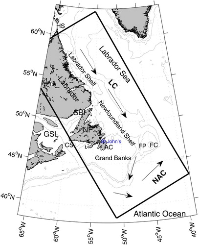
Fig. 2 Sites of moored measurements from 1979 to 2010 used in the model evaluation. The 200, 1000, and 3000 m isobaths are also shown. The two blue plus signs (sites A and B) indicate the locations where the model and observational current profiles are compared. The solid blue squares are monthly mean current observations at different depths. The open red circles and the red crosses are observational temperature sites at different depths over the Newfoundland Shelf and the Labrador Shelf, respectively. The solid red square indicates the location of Station 27 where temperature and salinity were observed. ST, BT, and FT are the Seal Island, Bonavista, and Flemish Cap Transects, respectively. The thick black line is the model boundary.
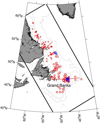
Fig. 3 32-year average model currents at 20 m below the surface in January and July, representing winter and summer. The 200, 1000, and 3000 m isobaths are also depicted in red, green, and black, respectively.
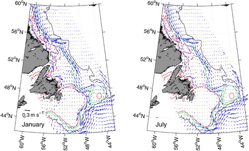
Fig. 4 Sub-sampled model currents at 20 m above bottom in January and July. The 200, 1000, and 3000 m isobaths are also depicted in red, green and black, respectively.
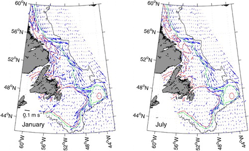
Fig. 5 Model sea-ice concentration of 0.1 south of 55°N in December and March, for the year with the median modelled sea-ice extent for 1979 to 2010. The observed areal sea-ice boundary with a sea-ice concentration of 0.1 (thick grey line) is also shown, for the year with the median observed sea-ice extent over the same period. The 1000 m isobath (solid line) is depicted.
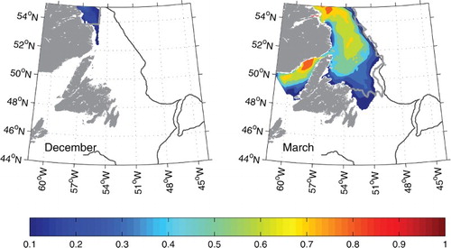
Fig. 6 Monthly sea surface (a) temperature and (b) salinity as well as bottom (c) temperature and (d) salinity at Station 27 from the model and observations.
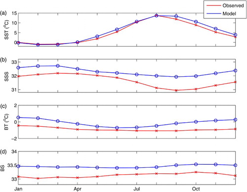
Fig. 7 Monthly observed and simulated temperatures at mooring stations over the Newfoundland Shelf for (a) 0–40 m, (b) below 40 m, and the Labrador Shelf for (c) 0–40 m and (d) below 40 m. Moorings locations are indicated in .
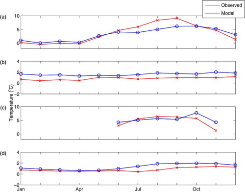
Fig. 8 Surface layer (solid line with squares) and bottom layer (dashed line with circles) for (a) temperature and (b) salinity for the Flemish Cap transect.
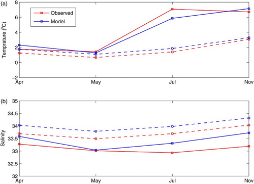
Fig. 9 As in , but for the Bonavista transect.
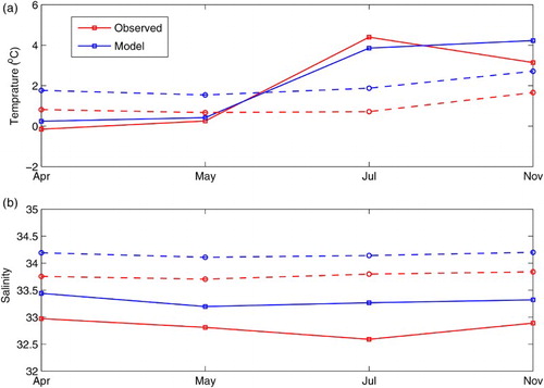
Fig. 10 Monthly mean depth-averaged currents in the Flemish Pass. Locations are indicated by solid blue squares in .
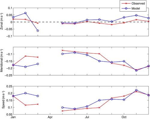
Table 1. Statistics comparing model currents and monthly mean observations in the Flemish Pass. Locations are shown in . U is the zonal velocity and V is the meridional velocity (m s−1).
Fig. 11 Comparison between selected model monthly mean current profiles and moored measurements. U and V are the zonal and meridional components, respectively. Red squares are observations and the blue lines are model results. See for the locations of sites A and B.

Table 2. Statistics comparing vertical profiles of monthly mean simulated currents and the monthly mean observations at sites A and B. Locations are shown in . U is the zonal velocity and V is the meridional velocity (m s−1).
Fig. 12 Comparison between the model currents with vessel-mounted ADCP data along the Flemish Cap transect in spring, summer, and fall. Only the normal component (m s−1; positive southward) is shown.
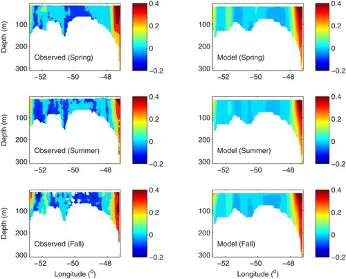
Table 3. Statistics comparing Flemish Cap transect currents and the observed values in spring, summer, and fall. Transect locations are shown in . Units are m s−1.
Fig. 13 Monthly sea-ice extent south of 55°N.
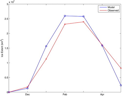
Fig. 14 Monthly volume transport (a) across the inshore portion, (b) across the upper slope, and (c) from the coast to the 3000 m isobath across the Seal Island transect. The annual mean transport is also depicted (black dashed line).
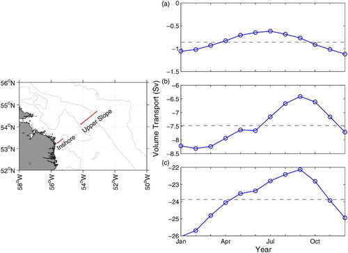
Fig. 15 Monthly volume transport (a) across the inshore portion, (b) through the Flemish Pass, and (c) from the coast to the 3000 m isobath across the Flemish Cap transect. The annual mean transport is also depicted (black dashed line).
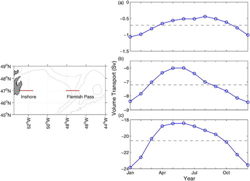
Fig. 16 Monthly freshwater transport (a) across the inshore portion, (b) across the upper slope, and (c) from the coast to the 3000 m isobath across the Seal Island transect. The annual mean freshwater transport is also depicted (dashed black line).
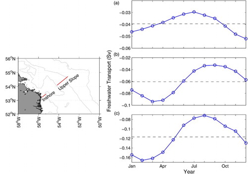
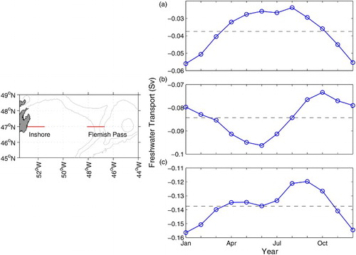
Fig. 17 Monthly freshwater transport (a) across the inshore portion, (b) through the Flemish Pass, and (c) from the coast to the 3000 m isobath at the Flemish Cap transect (47°N). The annual mean freshwater transport is also depicted (dashed black line).