Figures & data
Fig. 1 Map of the study area showing the model domain, with a small sub-area of the grid in the lower right corner. The 200 and 1000 m depth contours are shown. The blue arrows represent the position of the Anticosti Gyre (AG) and Gaspé Current (GC). The red dots show the locations of the five ADCP moorings (M1, M2, M3 (and its relocated position M3b), M4, and M5). The thick blue line shows the position of the Jacques-Cartier Strait transect (see inset for the model depths across the transect from the south towards the north). The thick blue line at the shelf break south of Newfoundland shows the location of the SB valve (i.e., where the shelf break transport was modified for the Cabot Strait transport sensitivity analysis). The eastern half of the Cabot Strait transect (Cabot-E) is also depicted with a blue line.
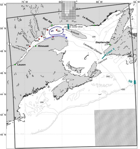
Fig. 2 Typical mean krill nighttime and daytime vertical distribution observed with the ADCP at station M4 in July 2009. The light grey line shows a modified daytime vertical distribution to simulate aggregation of krill near the bottom in areas shallower than 100 m.
Fig. 3 Mean 2006–2010 currents averaged over krill mean nighttime ((a) to (d) 0–40 m) and daytime ((e) to (h) 80–180 m) depths for each season. Blue arrows indicate westward-flowing currents and red arrows eastward-flowing currents.
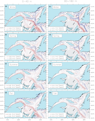
Fig. 4 Comparison of observed (blue) and simulated (red) daily mean currents over two layers, 10–40 m and 40–100 m, at stations M1, M2, M3, and M3b shown in . The current coordinate system was rotated by 15° to match the alongshore axis at M1, by 60° at M2, by 10° at M3, and by 30° at M3b (positive values indicate an eastward flow out except for M2 where they indicate a northward flow). The x-axis shows the time from October 2007 to November 2009. The greyed areas correspond to the events described in . The γ2 values calculated by Eq. (1) are also displayed in the upper left corner of each panel.
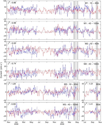
Fig. 5 GEM-simulated (blue line) versus observed (green line) monthly mean winds at 10 m at (a) Sept-Îles, (c) Baie-Comeau, and (e) Stephenville and (b), (d), and (f) air temperature at 2 m at the same locations. The red line on (a), (c), and (e) represents the absolute difference between observed and simulated winds. The location of the stations is displayed in , except for Baie-Comeau, which is displayed in . Wind and air temperature data were obtained from Environment Canada.
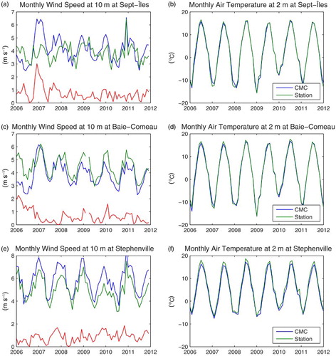
Fig. 6 Mean normal velocities (lines) and temperature (colours, °C) for the five-year period (2006–2010) simulated by the model for each season (Control run) at Cabot Strait. Positive (negative) values indicate outflowing (inflowing) currents, and distance 0 is the western side of the strait.
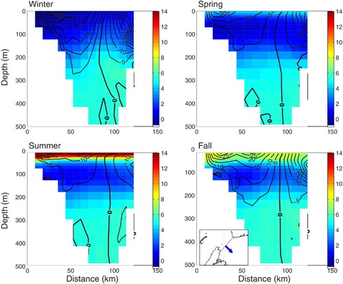
Fig. 7 Comparison of seasonal sea surface temperatures (in °C) between the satellite and the model (Control run) for 2009. The SST data are generated using NOAA Advanced Very High Resolution Radiometer (AVHRR) satellite images.
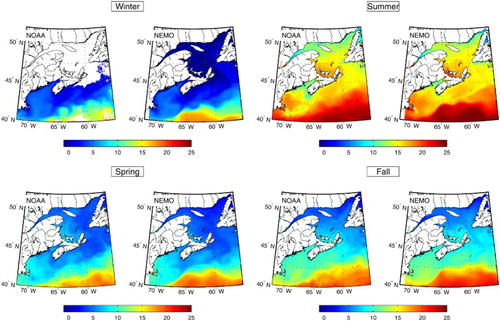
Fig. 8 Observed (conductivity, temperature, depth (CTD) sensor) and simulated (NEMO) monthly T-S diagrams of the water masses in the GSL in 2009 at corresponding locations, shown on map (colours), and times. Simulated water masses have the same composition as observed water masses. Temperature units on the y-axis are °C.
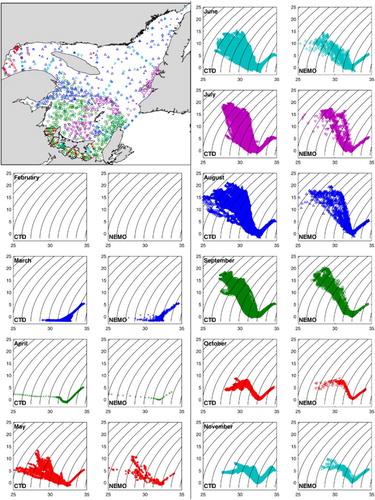
Table 1 RMSEs for salinity and temperature from the Control run in 2009 and the data presented in .
Fig. 9 Sea-ice concentration in February and March of 2009 and 2010, with (left) the Control run and (right) the weekly estimates from the Canadian Ice Service.
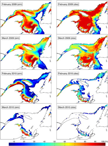
Fig. 10 Enlarged version of . Mean 2006–2010 currents averaged over krill mean nighttime ((a) to (d) 0–40 m) and daytime ((e) to (h) 80–180 m) depths for each season in the LSLE and nwGSL. The location of the PdM transect is displayed in (g), with the northern portion (nPdM) in grey and the southern portion (sPdM) blank. Blue arrows indicate westward-flowing currents and red arrows eastward-flowing currents.
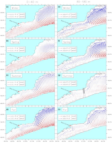
Fig. 11 Yearly time series of the seven-day moving average of (a) 0–40 m averaged transport across the nPdM cross-section, (b) transport across JCS, (c) transport across SBI, (d) transport at the eastern half cross-section of Cabot Strait, and (e) mean water level in the LSLE (between the Saguenay Fjord and PdM), for the five years of the simulation. The bold line on each panel is the five-year mean. The vertical line represents the approximate timing of the mean circulation shift. Negative transport denotes inward transport (i.e., westward).
Fig. 12 (a) North–south (thin line) and east–west (bold line) component of the mean winds over the GSL, north of Îles de la Madeleine (positive pointing north or east). Mean daily transport across the two PdM half sections (see g) in 2009, nPdM (thick line), and sPdM (thin line) and over three different layers: (b) 0–40 m, (c) 80–180 m, and (d) entire water column for the Control run and for the sensitivity analysis with constant runoff over the year for the large rivers flowing into the LSLE (SMOBSLcst, see Section 2d). The large negative pulses at nPdM are indicative of inflow events (grey shading), and the arrows point to the two inflow events detailed in .
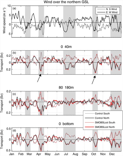
Fig. 13 Circulation and wind conditions during the two nPdM inflow events indicated by the arrows in and a no-inflow case on 2 May. (a), (b), and (c) Daily vertically averaged current for the surface layer (0–40 m) overlain on the surface salinity. The insets show current speed cross-sections across the PdM transect (negative values are upstream). (d), (e), and (f) Daily wind stress calculated by the atmospheric model and used to force the ocean circulation model overlain on the daily mean water level.
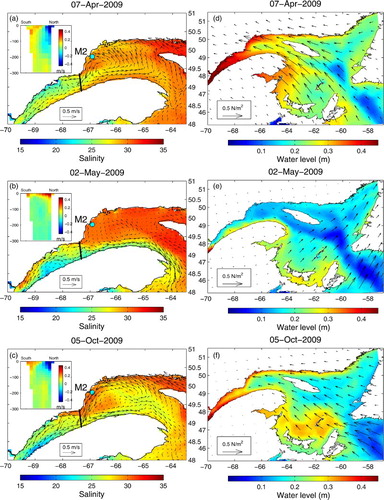
Fig. 14 Daily mean krill density at each grid cell (integrated number of particles from the surface to the bottom) at different times of 2009 for the DVM krill scenario (MIGR). The initial density on 1 December of the previous year was 400 individuals per horizontal cell.
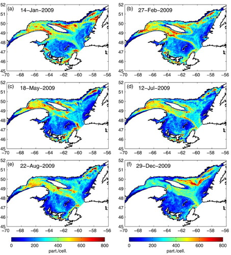
Fig. 15 Mean krill density (number of individuals per vertically integrated grid cell) in the LSLE (between the Saguenay Fjord and PdM) for each year and for the three vertical distribution scenarios (MIGR, DAY, and NIGHT) (a), (b), and (c) for the yearly simulations and (d), (f), and (e) for the five-year simulations, each year being represented separately for comparison with the yearly simulations. The initial density on 1 December of the previous year was 400 individuals per horizontal cell for the yearly simulations. The five-year run started on 1 December 2005. Note that the vertical scale of the DAY simulation is twice as large as for the other simulations. For the five-year DAY scenario (e), in which LSLE krill steadily accumulate, the krill density at the beginning of each year was brought down to 500 for the comparison (actual mean densities at the end of each year were 894, 1020, 1296, 1432, and 1509 individuals per grid cell for 2006 to 2010, respectively).
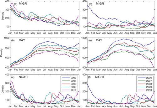
Fig. 16 Mean currents in the 0–40 m layer for the summer with (a) the Control simulation and the sensitivity analyses, (b) SMOBSLcst, (c) LowBI, (d) HighSB, and (e) SWwind, with the mean 0–40 m summer salinity colour mapped, as well as (f) the climatological (1971–2000) mean 0–40 m salinity.
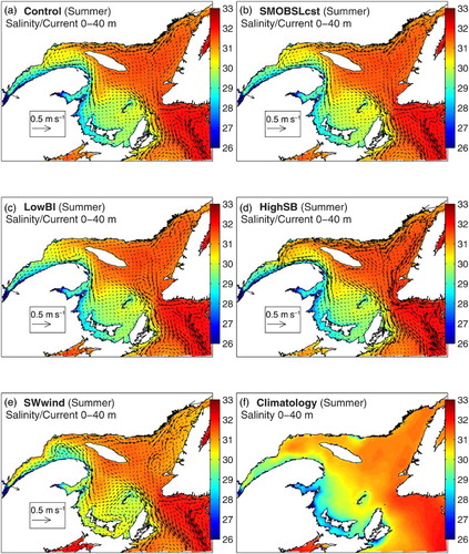
Fig. 17 As in , but showing only the five-year means for the Control simulation and the sensitivity analyses. Seven-day moving average of (a) transport across the nPdM cross-section averaged over the 0–40 m layer, (b) transport at JCS, (c) transport at SBI, (d) transport at the eastern half of Cabot Strait, and (e) mean water level in the LSLE (between the Saguenay Fjord and PdM. The vertical line represents the approximate timing of the mean circulation shift. Negative transport denotes inward transport (westward).
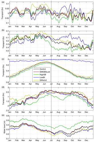
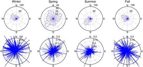
Fig. 18 Wind roses for each season for the northern GSL, (upper) total number of days with the wind blowing from each direction between 2006 and 2010, (lower) wind stress intensity from the corresponding directions.