Climate Comparisons and Change Projections for the Northwest Atlantic from Six CMIP5 Models

Figures & data

Table 1. Information on the six ESMs examined in the study. Grid sizes are presented as latitude x longitude. Further information can be obtained from the CMIP5 website (http://cmip-pcmdi.llnl.gov/cmip5/), the websites of the institutions which provided the model fields, or the references indicated.

Model Name	Institution	Reference	Atmospheric Grid	Oceanic Grid
CanESM2: Canadian Earth System Model, version 2	EC's Canadian Centre for Climate Modelling and Analysis (CCCma)	Arora et al. (2011)	∼2.8°	∼0.9° × 1.4°
GFDL-ESM2M: Geophysical Fluid Dynamics Laboratory's Earth System Model, version 2M	GFDL of the National Oceanic and Atmospheric Administration (NOAA, USA)	Dunne et al. (2012)	∼2° × 2.5°	0.3°–1°
HadGEM2-ES: Hadley Centre Global Environmental Model, version 2	Met Office Hadley Centre (United Kingdom)	Collins et al. (2011)	∼1.2° × 1.9°	0.3°–1°
IPSL-CM5A-LR: Low Resolution version of the Earth System Model based on the IPSL's Climate Model, version 5A	Institut Pierre-Simon Laplace (France)	Dufresne et al. (2013)	∼1.9° × 3.8°	0.5°–2°
MIROC-ESM: Earth System Model based on the global climate Model for Interdisciplinary Research on Climate	Japan Agency for Marine-Earth Science and Technology, Atmosphere and Ocean Research Institute (The University of Tokyo), and National Institute for Environmental Studies	Watanabe et al. (2011)	∼2.8°	0.5°–1.7° × 1.4°
MPI-ESM-LR: Low Resolution version of the Max-Planck-Institute Earth System Model	Max Planck Institute for Meteorology (Germany)	Giorgetta et al. (2013)	∼1.9°	∼1.6°

Fig. 1 (a) Map showing land areas (italics) and locations of the two sections (LSSS and SSSR) used for displays of subsurface temperature and salinity (blue lines); the seven model sites where temporal variability in SST and SSS is examined (red squares); and the ocean observation site (Station 27 or S27; green square) that is not collocated with the model site. (b) Map showing ocean areas (italics) and locations of the seven model sites (including six meteorological observation stations) where temporal variability in SAT is examined (red squares).

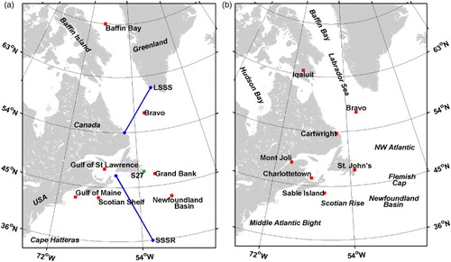
Fig. 2 Annual cycles of the bidecadal monthly means of SAT for 1986–2005 at six sites from observations (AHCCD, red; see Fig. 1b for locations) and from historical Run 1 of the six ESMs (see colour legend). The SD_o of the individual-year AHCCD monthly means about each bidecadal mean is indicated by the red error bar.

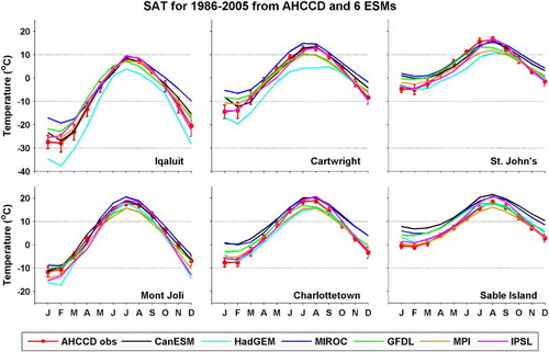
Fig. 3 Changes in bidecadal SAT for Canada from 1986–2005 to 2046–2065 from six ESMs for RCP8.5 in (a) February and (b) August. The ensemble mean, SD_m, and spread of the changes in (a) and (b) are shown in (c) for (top row) February and (bottom row) August. The white contours represent the 0°, 5°, and 10°C isotherms.

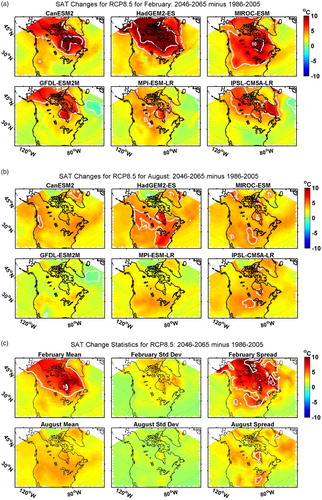
Fig. 4 Changes in bidecadal monthly SAT from 1986–2005 to 2046–2065 for RCP8.5 at six locations (shown in Fig. 1b) from Run 1 of the six ESMs.

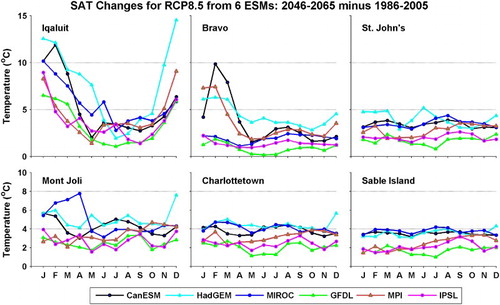
Fig. 5 (a) Comparison of SIC in March from the historical simulation (1986–2005) of each of six ESMs, the HadISST1 dataset for 1986–2005 (upper right), and the ensemble mean from the ESMs (only shown for grid points with values from all six ESMs). The differences in the apparent land areas (white) in the different models largely reflect differences in their native grids. (b) Ensemble-mean bidecadal monthly SIC for (left) January, (middle) March, and (right) May for 1986–2005 from (upper) the historical simulations and (lower) for 2046–2065 for RCP8.5 from the six ESMs (only shown for grid points with values from at least three ESMs). The grey contour in (b) represents the 30% isoline, approximating the ice edge.

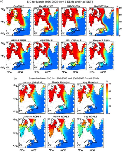
Fig. 6 Comparison of SST in February from the historical simulation of each of six ESMs for 1986–2005, the HadISST1 dataset for 1986–2005 (upper right), and the observed 0–10 m temperature climatology for 1946–2002 smoothed over an approximate 2° scale (for comparable resolution to the ESMs). The white contours represent the 2°, 10°, and 18°C isotherms.

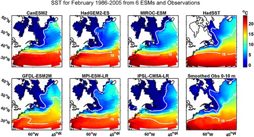
Fig. 7 Annual cycles of SST at the three DFO monitoring sites from observations (red; see Fig. 1a for locations) and for 1986–2005 from historical Run 1 of the six ESMs (see colour legend). The observed annual cycle for Bravo is from a harmonic fit to data over all years with an overall SD_o of 0.9°C (not shown on plot), and the cycles for the other sites are from monthly means for 1986–2005 with each vertical (red) bar indicating the SD_o of the individual-year means about the bidecadal mean.

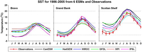
Fig. 8 Changes in bidecadal monthly SST from 1986–2005 to 2046–2065 for the NWA for RCP8.5 from the six ESMs (first three columns) for (a) February and (b) August. The ensemble mean, SD_o, and spread of the changes are also shown (last two columns) for grid points with values from at least three ESMs. The white contours represent the −4°, 0°, and 4°C isotherms.

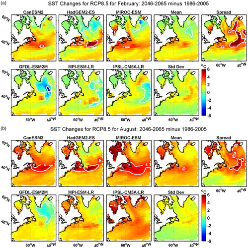
Fig. 9 Changes in bidecadal monthly SST from 1986–2005 (historical) to 2046–2065 (RCP8.5) at six sites in Fig. 1a for Run 1 of the six ESMs.

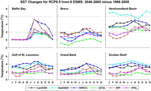
Fig. 10 Comparison of SSS in August from the historical simulation of each of six ESMs for 1986–2005, the observed 0–10 m salinity climatology for 1946–2002 on a 0.3° × 0.3° grid, and the climatology smoothed over an approximate 2° scale. The white contours represent the 33 and 35 isohalines.

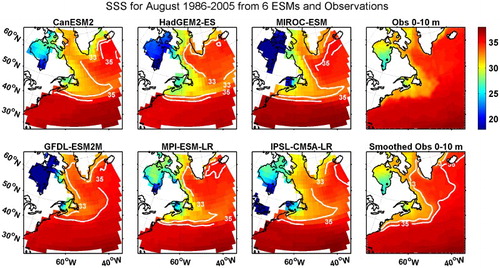
Fig. 11 Annual cycles of SSS at the three DFO monitoring sites from observations (red) and for 1986–2005 from historical Run 1 of the six ESMs. The observed annual cycle for Bravo is from a harmonic fit to data over all years with an overall SD_o of 0.2, and the cycles for the other sites are from monthly means for 1986–2005 with each vertical (red) bar indicating the SD_o of the individual-year means about the bidecadal mean.

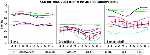
Fig. 12 Changes in bidecadal monthly SSS from 1986–2005 to 2046–2065 for RCP8.5 for August from the six ESMs (first three columns). The ensemble mean, SD_m, and spread of the changes are also shown for grid points with values from at least three ESMs. The grey contour represents the 0 isohaline.

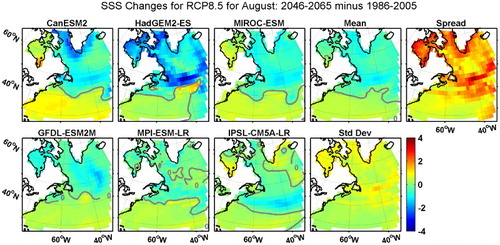
Fig. 13 Changes in bidecadal monthly SSS from 1986–2005 (historical) to 2046–2065 (RCP8.5) at six sites shown in Fig. 1a, in Run 1 from the six ESMs.

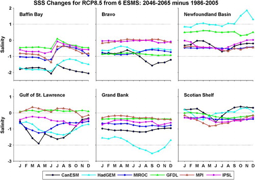
Fig. 14 Comparison of decadal means (1996–2005) of (a) potential temperature and (b) salinity across the LSSS section from five ESMs, with observations from the AR7W line over the period 1996–2008 (data from Yashayaev et al., 2014).

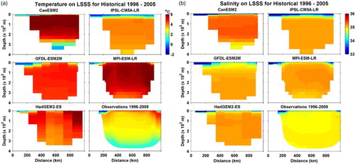
Fig. 15 Changes in bidecadal means of (a) potential temperature and (b) salinity from 1986–2005 (historical) to 2046–2065 (RCP8.5) on the LSSS section from five ESMs, with the 0 isolines shown in grey.

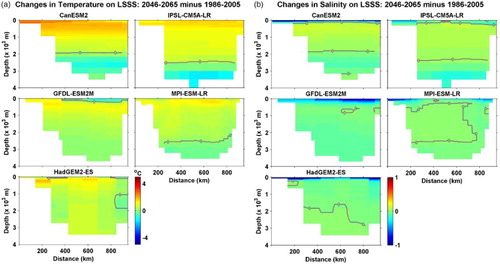
Fig. 16 Changes in bidecadal means of (a) potential temperature and (b) salinity from 1986–2005 (historical) to 2046–2065 (RCP8.5) on the SSSR section from five ESMs, with the 0 isolines shown in grey.

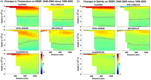
Fig. 17 (a) Bidecadal mean fields of OML-max in February from four ESMs for 1986–2005 from their historical simulations (top row) and for 2046–2065 from their RCP8.5 simulations (bottom row). The right panel in the top row shows an observational approximation to OML-max in February from Argo profiles during the 2002–2014 period. (b) Projected changes from 1986–2005 to 2046–2065 for the ESM fields in (a), with the 0 isoline shown in grey.

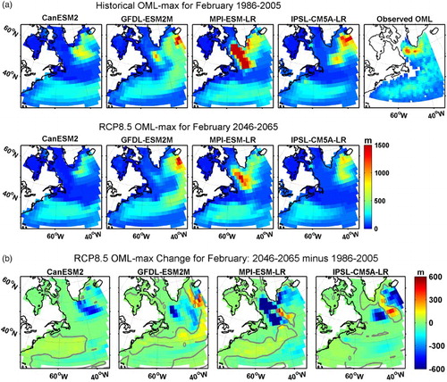
Fig. 18 Time series of annual means of (a) SAT and (b) SST at three nearby pairs of sites from the historical (1950–2005) and RCP8.5 (2006–2080) simulations of CanESM2 (five runs: R1–R5) and GFDL-ESM2M (1 run), with observed SAT and SST annual means included (up to 2011–2014 depending on site and variable). The nearby sites for SAT and SST, respectively, are Bravo in the Labrador Sea (top row), St. John's and the Grand Bank (second row), and Sable Island and the Scotian Shelf (lower row). See Figs. 1a and 1b for the specific locations.

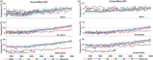
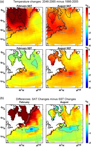
Fig. 19 (a) Changes in ensemble-mean SAT (top row) and SST (bottom row) from 1986–2005 (historical) to 2046–2065 (RCP8.5) for (left panels) February and (right panels) August (only shown for grid points with values from at least three ESMs). (b) Differences between the (ensemble-mean) SAT changes and SST changes for February and August shown in (a). The 0° and 3°C isotherms are shown in grey.

Arora, V. K., Scinocca, J. F., Boer, G. J., Christian, J. R., Denman, K. L., Flato, G. M.,  … Merryfield, W. J. (2011). Carbon emission limits required to satisfy future representative concentration pathways of greenhouse gases. Geophysical Research Letters, 38, L05805. doi:10.1029/2010GL046270

 Web of Science ®Google Scholar

Dunne, J. P., John, J. G., Adcroft, A. J., Griffies, S. M., Hallberg, R. W., Shevliakova, E., … Zadeh, N. (2012). GFDL's ESM2 global coupled climate–carbon Earth System Models. Part I: Physical formulation and baseline simulation characteristics. Journal of Climate, 25, 6646–6665. doi:10.1175/JCLI-D-11-00560

 Web of Science ®Google Scholar

Collins, W. J., Bellouin, N., Doutriaux-Boucher, M., Gedney, N., Halloran, P., Hinton, T., … Woodward, S. (2011). Development and evaluation of an Earth-system model – HadGEM2. Geoscientific Model Development, 4, 1051–1075. doi:10.5194/gmd-4-1051-2011

 Web of Science ®Google Scholar

Dufresne, J.-L., Foujols, M.-A., Denvil, S., Caubel, A., Marti, O., Aumont, O., … Vuichard, N. (2013). Climate change projections using the IPSL-CM5 Earth System Model: From CMIP3 to CMIP5. Climate Dynamics, 40(9–10), 2123–2165. doi:10.1007/s00382-012-1636-1

 Web of Science ®Google Scholar

Watanabe, S., Hajima, T., Sudo, K., Nagashima, T., Takemura, T., Okajima, H., … Kawamiya, M. (2011). MIROC-ESM 2010: Model description and basic results of CMIP5–20c3 m experiments. Geoscientific Model Development Discussions, 4, 845–872. doi:10.5194/gmd-4-845-2011

 Web of Science ®Google Scholar

Giorgetta, M. A., Jungclaus, J., Reick, C. H., Legutke, S., Bader, J., Böttinger, M., … Stevens, B. (2013). Climate and carbon cycle changes from 1850 to 2100 in MPI-ESM simulations for the Coupled Model Intercomparison Project 5. Journal of Advances in Modeling Earth Systems, 5(3), 572–597. doi:10.1002/jame.20038

 Web of Science ®Google Scholar

Yashayaev, I., Head, E. J., Azetsu-Scott, K., Wang, Z., Li, W. K. W., Greenan, B. J. W., … Punschon, S. (2014) Oceanographic and environmental conditions in the Labrador Sea during 2012. (Fisheries and Oceans Canada, Canadian Science Advisory Document Research Document, 2014/046). Retrieved from http://www.dfo-mpo.gc.ca/csas-sccs/Publications/ResDocs-DocRech/2014/2014_046-eng.html

 Google Scholar