Investigating the Effect of Oceanographic Conditions and Swimming Behaviours on the Movement of Particles in the Gulf of St. Lawrence Using an Individual-Based Numerical Model

Figures & data

Fig. 1 The model domain and its major bathymetric features. Abbreviations are used for Rivière-du-Loup (RdL), the St. Lawrence Estuary (SLE), Strait of Belle Isle (SBI), Prince Edward Island (PEI), and the Bay of Fundy (BoF). Black lines with circles indicate idealized channels that represent rivers in the model. The initial release area of particles is outlined with a solid red line in the SLE. The dashed red line at the mouth of the SLE indicates the location at which STST ceases. Atlantic Zone Monitoring Program (AZMP) stations are indicated by numbers, and tide gauges are indicated by letters.

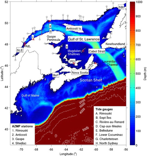
Fig. 2 Monthly-mean fields of salinity and currents for November 2011 calculated from model results at depths of (a) 5, (b) 20, (c) 50, and (d) 100 m in the St. Lawrence Estuary, Gulf of St. Lawrence, and eastern Scotian Shelf. Velocity vectors are shown at every fourth grid point. The dashed lines in (a) outline the area that will be shown in Fig. 3.

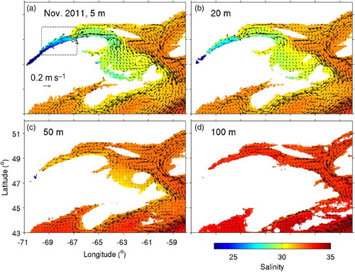
Fig. 3 Monthly-mean fields of salinity and currents for November 2011 calculated from model results at depths of (a) 5, (b) 20, (c) 50, and (d) 100 m in the St. Lawrence Estuary. Velocity vectors are shown at every model grid point.

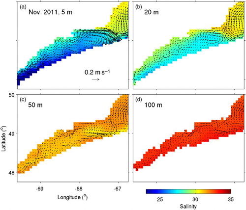
Fig. 4 (a) The life cycle of the American eel. Spawning takes place in the Sargasso Sea, and the larvae (leptocephali) are transported by ocean currents towards the east coast of North America. The juveniles (glass eels) migrate into coastal and inland waters and eventually metamorphose into yellow eels. During their seaward spawning migration, they metamorphose into silver eels. (Image reproduced by permission of the American Eel Monitoring Program at the Virginia Institute of Marine Science (http://www.vims.edu/research/departments/fisheries/programs/eel_survey/life_history/index.php). (b) Depth recorded every 15 minutes by an electronic tag attached to a silver American eel, released from Rivière-du-Loup in the SLE (Fig. 1). This dataset was also used in Fig. 2 of Béguer-Pon et al. (2012).

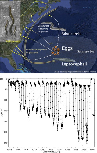
Fig. 5 Scatterplots between observed and simulated amplitudes and phases of tidal elevations for the M₂ and K₁ tidal constituents for 2011 at the eight tide gauge locations shown in Fig. 1.

Fig. 6 Scatterplots between simulated and observed salinity for 2011 at AZMP stations: (a) Rimouski, (b) Anticosti, (c) Gaspé, and (d) Shediac.

Fig. 7 Schematic diagram for the manner in which the numerical particle-tracking scheme moves particles that have moved into a dry grid cell of the model back to a wet grid cell. The grey squares represent wet grid cells, and the white squares represent dry grid cells. (a) The particle is in cell 1 (a wet grid cell) at time t (at the position denoted by a square), but its calculated position for time t+Δt (denoted by a circle) is in cell 3 (a dry grid cell); (b) the particle-tracking scheme determines that the closest grid cell to the particle's provisional new position is cell 4, followed by cell 1; (c) however, the particle cannot move into cell 4 because it also is a dry grid cell; and (d) the particle moves northward into cell 1, and its new meridional distance from the coast (Δy₂) is of the same magnitude as the meridional distance by which it had moved inland in the provisional position (Δy₁).

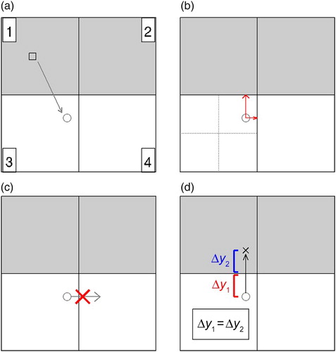
Table 1. Sunrise and sunset times used in experiments that include DVM.

Dates	Sunrise	Sunset
19 October–6 November	1100 utc (0600 local time)	2200 utc (1700 local time)
7 November–1 December	1100 utc (0600 local time)	2100 utc (1600 local time)
2 December–3 February	1200 utc (0700 local time)	2100 utc (1600 local time)

Table 2. List of the 19 numerical experiments conducted in this study. In experiments H1, H2, S1, S2, and W1, the lateral swimming speed is 0.5 m s⁻¹. The experiments are grouped as follows: Group A (experiments P1, P2, P3, P4, HM1, HP1, VM1, VP1, P1H, and P1D), Group B (experiments M1, M2, M3, and T1), and Group C (experiments H1, H2, S1, S2, and W1).

Experiment	Description
Group A
P1	Passive, released 20 m from surface, movement due to advection and subgrid-scale processes
P2	Similar to P1 but released 20 m above bottom or 90% of water depth if water depth <60 m
P3	Similar to P1 but with no vertical advection
P4	Similar to P2 but with no vertical advection
HM1	Similar to P1 but with horizontal eddy diffusivity set to 0.1 times the default value
HP1	Similar to P1 but with horizontal eddy diffusivity set to 10 times the default value
VM1	Similar to P1 but with vertical eddy diffusivity set to 0.1 times the default value
VP1	Similar to P1 but with vertical eddy diffusivity set to 10 times the default value
P1H	Similar to P1 but with release time of particles varied by up to 12 hours before and after default time, in one-hour increments
P1D	Similar to P1 but with release time of particles varied by up to 360 hours (15 days) before and after default time, in 24-hour increments
Group B
M1	Including DVM with upper limit (zs) set to 20 m below sea surface and lower limit (zd) set to 20 m above sea bottom or 90% of water depth if water depth <60 m. Particles cannot move below 300 m depth. Lateral movement is passive (similar to P3 and P4)
M2	Similar to M1 but with upper limit (zs) set to 5 m below the sea surface
M3	Similar to M1 but with lower limit (zd) set to 5 m above sea bottom for water depth >60 m
T1	Including DVM and STST with upper limit for both (zs) set to 20 m below sea surface and lower limit for both (zd) set to 20 m above sea bottom or 90% of water depth if water depth < 60 m. Lateral movement is passive
Group C
W1	Including DVM and STST as defined in T1 and, outside the SLE, lateral swimming in random directions generated every hour
H1	Including DVM and STST as defined in T1 and, outside the SLE, lateral swimming towards deeper water (up to 300 m depth) if found among surrounding model grid points. Search for deeper water occurs every hour during the day. If none is found or if it is night, lateral swimming in random direction generated every hour
H2	Similar to H1 but with search for deeper water occurring every other hour during the day
S1	Including DVM and STST as defined in T1 and, outside the SLE, lateral swimming towards higher salinity if found among surrounding model grid points. Search for higher salinity occurs every hour during the night. If none is found or if it is daytime, lateral swimming in random direction generated every hour
S2	Similar to S1 but with search for higher salinity occurring every four hours during the night

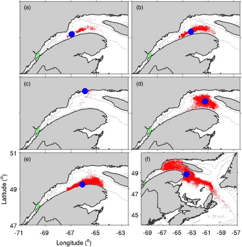
Fig. 8 Distributions of particles after 60 days in (a) experiment P1 (passive particles released at 20 m depth), (b) experiment P2 (passive particles released near the bottom), (c) experiment P3 (similar to P1 but with no vertical advection), (d) experiment P4 (similar to P2 but with no vertical advection). The blue circle indicates the location of the centre of mass of the particles, and the area outlined in green represents the release area for the particles.

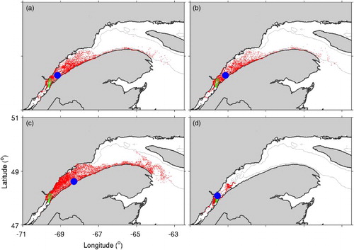
Fig. 9 Means (circles) and standard deviations (crosses) for (a) horizontal distances of particles relative to the centre of mass and (b) depths of particles after 60 days, in experiments P1 to P4 and the experiments in group B (in which the horizontal eddy diffusivity of the random walk component is decreased (HM1) or increased (HP1) by an order of magnitude, or the vertical eddy diffusivity is decreased (VM1) or increased (VH1) by an order of magnitude.)

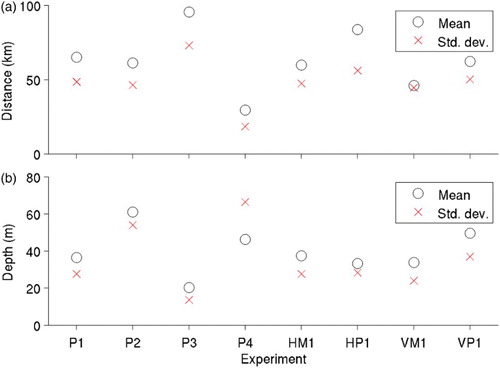
Fig. 10 Means (circles) and standard deviations (crosses) for (a) horizontal distances of particles relative to the centre of mass and (b) depths of particles, in experiment P1H (passive particles with release times varied in one-hour increments, up to 12 hours, before and after the release time used in experiment P1); (c) and (d) are similar to (a) and (b) but for experiment P1D (similar to experiment P1H but with particle release times varied in one-day increments, up to 15 days, before and after the release time used in experiment P1).

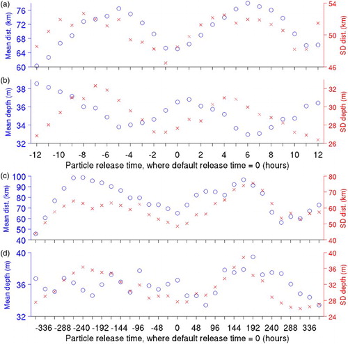
Fig. 11 Distributions of particles after 60 days in (a) experiment M1 (the upper limit of DVM is the 20 m depth and the lower limit is 20 m above the bottom or 90% of the water depth if the water depth < 60 m); (b) experiment M2 (the upper limit of DVM is changed to the 5 m depth); (c) experiment M3 (the lower limit of DVM is changed to 5 m above the bottom if the water depth is > 60 m); and (d) experiment T1 (DVM is the same as in experiment M1, but STST is added). The blue circle indicates the location of the centre of mass of the particles and the area outlined in green represents the release area of particles.

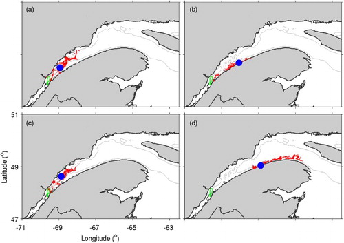
Fig. 12 Distributions of particles after 60 days in (a) experiment H1 (when outside the SLE, particles search for surrounding model grid points with deeper water every hour during the day and swim towards it if one is found; otherwise, they swim in random directions); (b) experiment H2 (similar to H1 but searching for deeper water every other hour during the day); (c) experiment S1 (when outside the SLE, particles search for surrounding model grid points with higher salinity every hour during the night and swim towards it if one is found; otherwise, they swim in random directions); (d) experiment S2 (similar to S1 but searching for higher salinity every four hours during the night); and (e) experiment W1 (particles swim in random directions during all hours when outside the SLE). (f) Distribution of particles after 120 days in experiment W1.

Table A1. List of major rivers in the St. Lawrence Estuary and Gulf of St. Lawrence, station names, and years of observation periods.

Status in the model	River name	Station name	Year(s) of observations used
Updated Rivers	St. Lawrence	Québec	2011
	Moisie	02UC002	1966–2012 excluding 1967, 1999, 2000, 2002, and 2006
	Romaine	02VC001	1957–2012 excluding 1960, 2002, and 2007
	Petit Mécatina	02XA008	1995 and 1998–2012 excluding 2005–2006
	Saint-Paul	02XC001	1968–2012 excluding 1972, 1981, 1990, 1996–1999, 2002, and 2005–2006
	Restigouche	01BJ007	1969–2012
New Rivers	Saguenay	02RH019	1943–1993
	Betsiamites	02SB004	1964–1994 excluding 1990
	Outardes	02TE001	1923–1977 excluding 1929–1931
	Manicouagan	02TC001	1947–1979
	Matane	02QB001	1927–2012 excluding1940
	Nabisipi	02WA001	1963–1987
	Aguanus	02WA002	1963–1981
	Humber	02YL003	1983–2013

Béguer-Pon, M., Benchetrit, J., Castonguay, M., Aarestrup, K., Campana, S. E., Stokesbury, M. J., & Dodson, J. J. (2012). Shark predation on migrating adult American eels (Anguilla rostrata) in the Gulf of St. Lawrence. PLoS ONE, 7(10), e46830, 1–11. doi:10.1371/journal.pone.0046830

 Web of Science ®Google Scholar