Variability of Current Streams in Atlantic Canadian Waters: A Model Study

Figures & data

Fig. 1 Schematic of the circulation in the study region. See Table 1 for abbreviations used in figure. Blue (red) arrows denote cold (warm) current streams. The red dot denotes Halifax. The flow through Flemish Pass is illustrated by a dashed arrow.

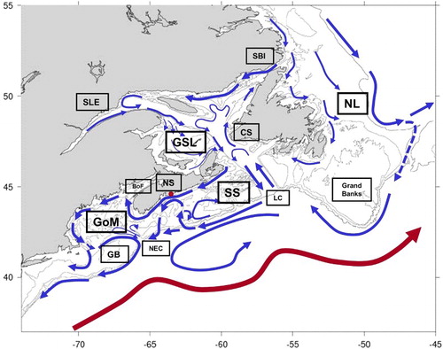
Fig. 2 Sections analyzed in this study (thick red lines). See Table 1 for abbreviations used in figure. The Flemish Cap section was broken into Flemish Pass (Fp) and Flemish Cap (Fc) subsections. Isobaths are shown at 50, 100, 200, 300, 500, 1000, and 2000 m. The 1000 m isobath is in bold, the 2000 m isobath is dashed, and the 100 m isobath is blue.

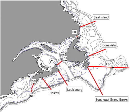
Table 1. Key section and place names and their abbreviations.

Name	Abbreviation
Seal Island	SI
Strait of Belle Isle	SBI
Bonavista	BV
Flemish Pass	Fp
Flemish Cap	Fc
southeast Grand Banks	se-GB
Cabot Strait	CS
Louisbourg	Lb
Halifax	Hfx
Cape Sable Island	CSI
Northeast Channel	NEC
Newfoundland and Labrador	NL
Gulf of St. Lawrence	GSL
Laurentian Channel	LC
Scotian Shelf	SS
Bay of Fundy	BoF
Gulf of Maine	GoM
Georges Bank	GB
St. Lawrence Estuary	SLE
Nova Scotia	NS

In the text nearshore and shelf break subsections are denoted by “:inner” and “:sb” appendices, respectively.

Fig. 3 Example of seasonal cycle fits showing (a) seasonal cycle behaviour at the inner part of the Louisbourg section and (b) no seasonal cycle behaviour at the shelf break of the Louisbourg section. The dashed blue lines are the raw data; red lines are the mean of the raw data; and the black lines are the model fits.

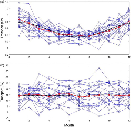
Fig. 4 Circulation and streamlines based on model climatological depth-averaged flow field. Streamlines selected to illustrate the various pathways from the northern Labrador Shelf to the south and west. See text for details. Isobaths as in Fig. 2.

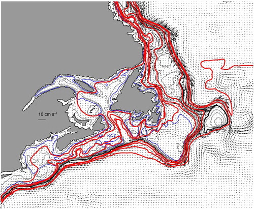
Fig. 5 Summary of seasonal cycle analysis. The green (red) arrows denote locations with (without) seasonal cycles; the question mark denotes an uncertain result. The dashed lines connecting the arrows are based on model velocity field streamlines.

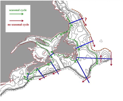
Table 2. Seasonal cycle fit for the 0–500 m depth bin.

Section	Transport	Amplitude	Phase	Std (phase)
SI:inner	2.37	0.58	5.52	0.71
SI:sb	16.36	0.82	5.62	1.47
SBI:net	0.16	0.08	5.82	1.09
BV:inner	2.04	0.48	6.37	0.53
BV:sb	10.69	0.59	5.12	1.64
Fp:inner	1.27	0.41	6.15	0.84
Fp:sb	8.44	1.02	5.11	1.27
Fc:west	−0.33	0.25	5.78	1.66
Fc:sb	6.25	1.01	5.81	1.87
se-GB:inner	1.38	0.42	6.10	0.85
se-GB:sb	5.26	3.27	5.97	1.60
CS:net	0.19	0.08	5.83	1.19
CS:outflow	0.67	0.27	5.73	0.86
CS:inflow	−0.49	0.20	5.92	0.88
Lb:inner	0.56	0.24	6.65	1.32
Lb:sb	4.36	1.93	5.98	1.86
Hfx:inner	0.68	0.24	6.92	0.82
Hfx:sb	4.77	1.19	6.53	1.94
CSI:inner	0.23	0.13	6.52	1.34
NEC:inflow	0.24	0.10	7.29	1.18
NEC:outflow	−0.26	0.12	7.08	1.41

Results are averages of the 22 estimates. The transport and amplitude are in Sv; phase is adjusted to be the month of the minimum in the cycle; standard deviation of the phase (std(phase)) is in months. Locations deemed to be without a seasonal cycle are in bold std(phase) values. Transports are positive for flow in the general northeast–southwest direction and negative for transports in the opposite direction. Fc:west and Fc:sb denote the western and eastern flanks of Flemish Cap. See Table 1 for other abbreviations.

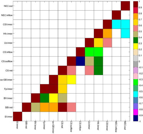
Fig. 6 Colour-coded correlations of shelf-break series at the 90% confidence level. Note that the colour scale is 0 to 1.

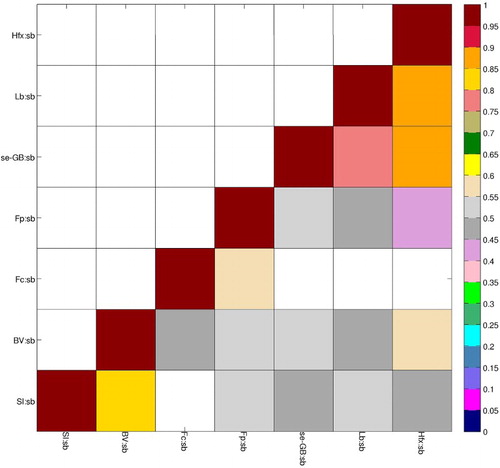
Fig. 7 Colour-coded correlations of the onshelf series at the 90% confidence level. Note that the colour scale is −1 to 1.