Figures & data
Fig. 1 Model domain (light grey area) including bathymetry, rivers (green circles), and storm surge locations of interest (red stars). The black rectangle represents the region displayed in .
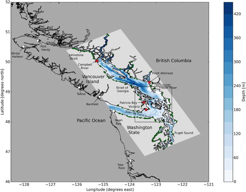
Fig. 2 Model bathymetry and coastlines in the passages between the San Juan and Gulf Islands. See for an explanation of the red stars.
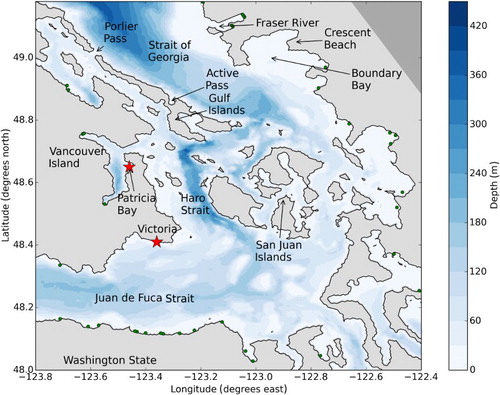
Table 1. Average peak surge amplitudes and delay in peak timing from Tofino at several tide gauges on the Pacific coast. Averages obtained over the five surge events hindcast in this article. A negative delay indicates that the peak surge occurred later than at Tofino.
Fig. 3 Evaluation of model tidal amplitude and phases for the M2 and K1 constituents. On the left, a transect through the stations used for comparison. On the right, (top) modelled M2 (black) and K1 (grey) amplitude and (middle) phase compared with observations in the dashed curves of the same colour. The bottom plot displays the M2 and K1 complex differences. Station names and numbers are listed in of Appendix A.
Table 2. Evaluation of model performance for all hindcasts presented. Mean absolute error ( ), observed mean (subscript o), modelled mean (subscript m), , and the Willmott skill score () are provided for water level predictions () and residuals (). Statistics are calculated over the time period displayed in each simulation's corresponding figure (three or four days). For the November 2006 case, the statistics were calculated over a three-day period. The average values were calculated over all the hindcasts, excluding the December 2012 HRDPS simulation.
Table 3. Summary of maximum water level, maximum surge amplitude, and model delay for all simulations. The model time delay is the number of hours between the maximum in the observations and the maximum in the model. A negative number means the model's maximum was later than the observations. Values are calculated over the same periods discussed in .
Fig. 4 Comparison of observations and model output for the 4 February 2006 storm surge. (Left) total water level observations (solid) and corrected model (dashed). (Right) observed residuals (solid) and modelled residuals (dashed).
Fig. 5 Comparison of the modelled residual for four simulations in February 2006: A simulation with all forcing (solid black), a simulation without local atmospheric forcing (dashed green), a simulation without remote forcing (solid red), and a simulation with only tides and local wind forcing (i.e., no remote forcing or local atmospheric pressure) (dashed blue).
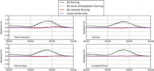
Fig. 6 Modelled residuals (solid line) compared with a simulation of the surge propagation without tidal forcing (dashed line) for the February 2006 hindcast.
Fig. 7 Spatial dependency of tide–surge interaction in the February 2006 hindcast. Differences in sea surface height between simulations with tidal forcing and without tidal forcing. Each plot is an average over 4 hr.
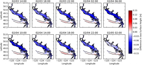
Fig. 8 Comparison of observed and modelled water level and residuals during the 15 December 2006 storm surge simulation.
Fig. 9 Propagation of the storm surge on 15 December 2006. Modelled residual every hour starting at 0230 UTC 15 December. Time advances from top left to bottom right. Wind vectors from the atmospheric forcing are overlaid in black.
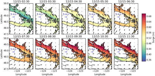
Fig. 10 As in , but for a simulation that does not include atmospheric forcing.
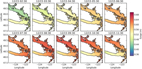
Fig. 11 Wind and storm surge conditions at Point Atkinson for a strong wind event on 19 November 2009. (top) Wind speed from Environment Canada observations (Environment Canada, Citation2014a) at Point Atkinson (solid line) and from the atmospheric model (CGRF) at a grid point near Point Atkinson (dashed line). (middle) Sea surface height anomaly at Tofino (solid line) and Port Hardy (dashed line) used as forcing conditions at the western and northern open boundaries. (bottom) Observed (solid line) and modelled (dashed line) residuals at Point Atkinson.
Fig. 12 Comparison of observed and modelled winds during the December 2012 storm surge simulation at (top) Point Atkinson, (middle) Sandheads, and (bottom) NOAA Buoy 46087. Observed winds are shown in solid black, low-resolution CGRF model in dashed black, and high-resolution model in grey. Observations from Sandheads and Point Atkinson are from the Environment Canada Climate Data archives (Environment Canada, Citation2014a). Observations at the NOAA Buoy were downloaded from http://www.ndbc.noaa.gov/stationpage.php?station=46087. Wind direction represents the direction that the wind is headed.
Fig. 13 Comparison of observed (solid black line) and modelled residuals for the December 2012 storm surge simulation. Modelled residuals from two simulations using low-resolution (dashed line) and high-resolution (grey line) atmospheric products are shown.