Figures & data
Table 1. Estimated amplitudes and phases for lines in the M2 Group.a
Fig. 1 Yearly estimates of the M2 tide deduced from hourly measurements taken at the tide gauge at Churchill on the western shore of Hudson Bay (top panel: amplitudes; bottom panel: Greenwich phase lags). In recent years the amplitude has been dropping markedly, while the phase lags have been increasing slightly. There is a small residual 18.6-year nodal modulation apparent in the phases. (Examination of the data residuals from the anomalous year 1967 suggests that that year's estimates are corrupted by timing errors during certain periods; also, the months April and December were completely missing).
Fig. 2 Yearly estimates of the K1 tide at Churchill.
Fig. 3 Yearly estimates of the M4 tide at Churchill. Unlike semi-diurnal constituents, the amplitude of M4 has tended to increase over the last two decades.
Fig. 4 Monthly estimates of the M2 tide at Churchill, obtained by repeated response analyses. Amplitudes H shown in red; Greenwich phase lags G shown in blue. In addition to the long-term decline, the amplitudes now show a suppressed seasonal cycle.
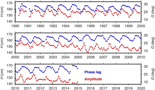
Fig. 5 Linear trends over the 2000–2014 interval in monthly estimates of the M2 tide at Churchill, separated according to month of observation. Amplitude H (centimetres per decade) in red; phase lags G (degrees per decade) in blue. Error bars (1−σ) account for autocorrelation in the residuals of fit. Amplitude trends are negative for all months, and they are most significantly negative in those months for which satellite altimeter data are available offshore.
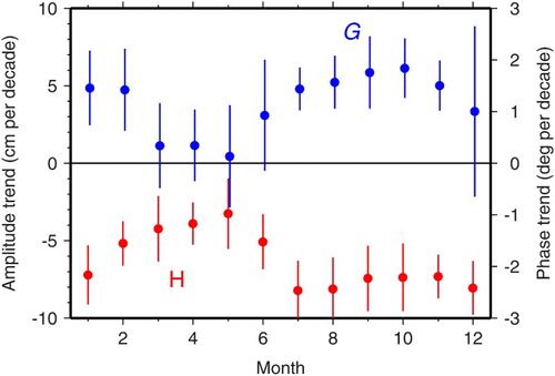
Fig. 6 Ground track locations of the T/P and Jason series of satellites, colour coded to the percentage of Jason-1 passes returning valid ocean data. (Percentages are similar for T/P and Jason-2.) Crossovers A through E are locations where the tides have been estimated from the altimeter data of each separate mission (T/P, Jason-1, and Jason-2); see .
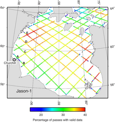
Fig. 7 Number of valid ocean altimeter returns obtained in each calendar month by the Jason-1 altimeter at the five crossover locations (A–E) shown in . These locations are mostly ice free only in the months July through October. No valid data at all are returned during January through April.
Fig. 8 Quality of altimeter tide estimates at crossover location E as a function of length of the altimeter time series (where “years” actually means ice-free seasons). The solid line is the standard error (cm) of M2 tidal estimates; the dashed line is the largest (absolute) correlation between estimated parameters, which is generally between constituents P1 and K2 (discounting Sa with itself).
Table 2. Estimates of M2 from altimetry at crossover locations.
Fig. 9 Annual mean high and low water (cm), shown after removal of the 18.6-year nodal cycle. Both MHW and MLW are decreasing over most of the time span, a reflection of the large glacial isostatic adjustment at Churchill. The decrease in the amplitude of the M2 tide since the 1990s coincides with MLW levelling off. The time series of high and low water was computed from the hourly data by employing a modified cubic spline (Ellis & McLain, Citation1977) for the required interpolations.
Fig. 10 Average monthly discharge rates (m3 s−1) of the Churchill River at hydrological station Red Head Rapids (58°70′7′′N, 94°37′20′′W). The large drop during the mid-1970s was caused by a major river diversion project after which most of the Churchill River was ultimately diverted into the Nelson River (Tushingham, Citation1992).