Figures & data
Fig. 1 (a) Northwest North Atlantic bathymetry (m) and Atlantic Canada Model (ACM) domain (outlined and in inset). (b) The model domain is divided into sub-areas for analysis: East of Newfoundland (ENfld), Grand Banks (GB), Gulf of St. Lawrence (GSL), Scotian Shelf (SS), Gulf of Maine (GOM), Offshore-south (OffS) and Offshore-east (OffE).
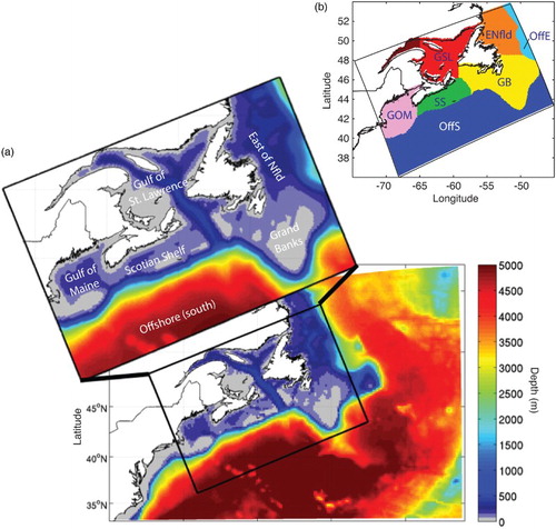
Table 1. Summary of external datasets providing atmospheric surface forcing data (CORE, NARR, ECMWF, ECMWF-EVAP) or ocean nesting data (HYCOM, MERCATOR, UBS).
Table 2. Atlantic Canada model (ACM) simulations.
Fig. 2 Time series of SST and SSS, averaged over (a) the entire ACM domain and (b) sub-areas from simulations with varied surface forcing (ACM-ECMWF, ACM-NARR, and ACM-CORE), with time series of climatology (grey dashed line) and satellite SST (grey stars) for comparison.
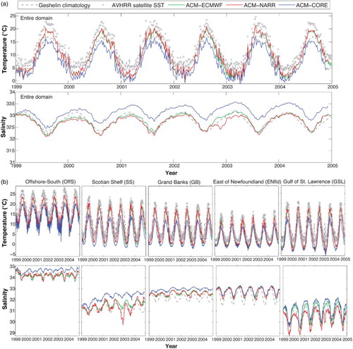
Fig. 3 Mean annual SSS anomaly (model-climatology) in 2003.
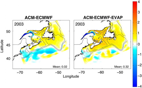
Fig. 4 Model salinity along the Halifax Line transect, overlain by AZMP observations, in May 2004, for three simulations: ACM-HYCOMdebias, ACM-MERCATORdebias, and ACM-UBS.
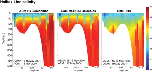
Fig. 5 Annual mean surface velocity (m s−1) mapped in 2004 for each simulation with varying ocean nesting (ACM-UBS, ACM-UBSclim, ACM-MERCATOR, ACM-MERCATORdebias, ACM-HYCOM, and ACM-HYCOMdebias). Vector arrows (black) are drawn at identical locations for comparison.
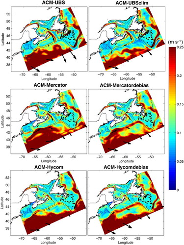
Fig. 6 The observed range of mean annual GSNW index locations (black outline with grey shading) (see in Joyce et al., Citation2000) with the long-term mean position of the ACM simulations (coloured lines) with (a) varied ocean nesting and (b) varied treatment of buffer zone nudging. The grey dashed line indicates the model grid boundary.
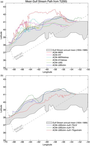
Fig. 7 (a) Section locations for model long-term mean volume transport comparison to the estimated mean annual transport listed by Loder et al. (Citation1998). LC1, GB1, GB2, and SF2 correspond to their Hamilton Bank, Flemish Pass, Tail of the Grand Banks, and Halifax Section, respectively (see their and .2). (b) Long-term mean volume transport (Sv) from model simulations with varied ocean nesting, and (c) from model simulations with varied nudging and grid size (sections shown in map in a).
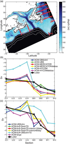
Fig. 8 (a) Time series of the total sea level from the Fisheries and Oceans Canada dataset (blue), the tidal component estimated using T_TIDE from Pawlowicz et al. (Citation2002) (green), and the non-tidal sea level (equivalent to the residual, red) (m) at the Halifax station for a 1-week period starting 26 March 1999. (b) Time series of the non-tidal sea level estimated from the Fisheries and Oceans Canada dataset (red) and in the model simulation ACM-UBSclim (blue) for the time period 1999–2001, with statistical results indicated in the inset (γ2, RMSE, the average absolute difference (AAD), and correlation r, following the definitions of γ2 and AAD of Zhang and Sheng (Citation2013)). Comparison of RMSE (m) for (c) all simulations at Halifax station, and (d) ACM-UBSclim at all stations (Rimouski, Saint-Francois, Sept-Îles, Charlottetown, Yarmouth, and Halifax).
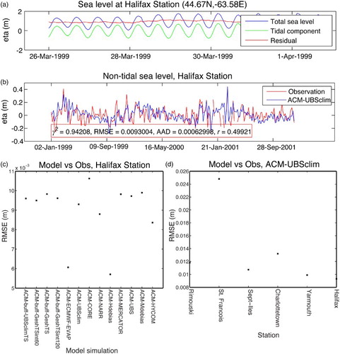
Fig. 9 Simulated and observed salinity at AZMP Station 27 (indicated on inset map) for the period 1999–2004. Root-mean-square error (RMSE) is reported for ACM-UBSclim (left) and ACM-buffGeshTS (right).
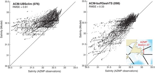
Fig. 10 (a) Model domain with bathymetry (m) for original and large grids, and (b) time series of area-averaged Scotian Shelf properties T (left) and S (right) at sea surface (upper) and bottom (lower) from model simulations ACM-orig (pink) and ACM-large (black), with comparison to climatology (grey dashed line) and AVHRR satellite SST (grey stars).
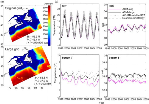
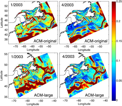
Fig. 11 Monthly-mean surface velocity (m s−1) in ACM-original (top) and ACM-large (bottom) in January 2003 (left) and April 2003 (right).