Figures & data
Fig. 1 Oxygen concentration (O2; μmol kg−1) on the 26.75 neutral density surface in the Pacific Ocean. A neutral density is a seawater potential density whose reference surface varies continuously with pressure (Ivers, Citation1975; Jackett & McDougall, Citation1997). The depth of this neutral density surface ranges from near zero in the northwest Pacific Ocean and zero in the Southern Ocean to about 300 m off Central America. Figure from WOCE Pacific Ocean Atlas by permission (Talley, Citation2007; http://www-pord.ucsd.edu/whp_atlas/pacific_index.html).
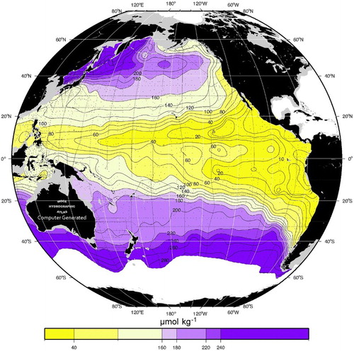
Fig. 2 Hovmöller graph of O2 sample locations on the 26.7 σθ surface of the continental slope where the bottom depth is between 210 and 1500 m. Regions shaded yellow denote latitude bands selected to examine trends in O2 on the continental slope from 36° to 49°N.
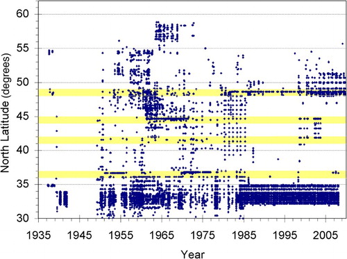
Fig. 3 Spatial distribution of O2 samples interpolated onto the 26.7 σθ surface in the Northeast Pacific Ocean, by decade. Red lines show locations of deep-sea sections and lines discussed: (c) 149.5°–161.5°W; (d) WOCE line P1 along 47°N; (e) Line P with stations P8, P12, P16, P20, and OSP each marked with a red asterisk, progressing from east to west; (f) section along northern end of WOCE line P17.
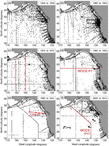
Fig. 4 Locations of CalCOFI stations off southern California from the 1990s to present. Blue arrows and numbers denote stations examined in our analyses (CalCOFI, Citation2015).
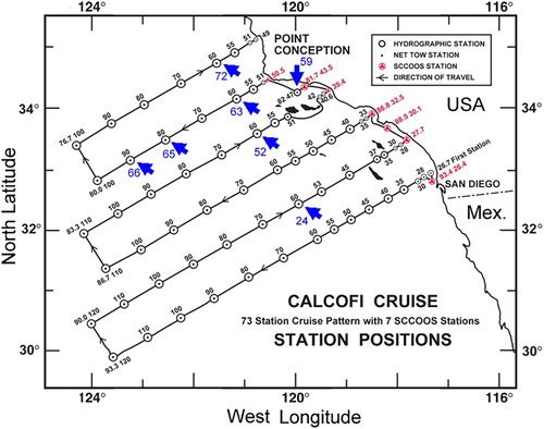
Table 1. CalCOFI stations discussed in this paper. Cross-slope (59, 63, 65, and 66) and along-slope (24, 52, 63, and 72) station locations are identified in .
Fig. 5 Scatterplots of observations of O2 (left, μmol kg−1) and Θ (middle, °C) interpolated onto the 26.7 σθ surface at four CalCOFI stations. Depth of the 26.7 σθ surface is plotted in the right column. Blue symbols represent individual observations. Red lines are significant quadratic polynomials of annual averages of O2. Black lines are best-fit quadratic polynomials to all observations of Θ and depth of the 26.7 σθ surface. Horizontal axes show the year of observation.
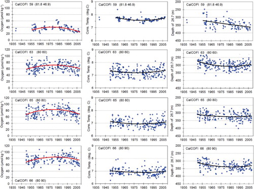
Fig. 6 Scatterplots of observations of O2 (left, μmol kg−1) and Θ (middle, °C) interpolated onto the 26.7 σθ surface, for locations on the continental slope between 36°N (bottom panels) and 49°N (top panels) where the bottom depth is between 210 and 1500 m. Depth of the 26.7 σθ surface is plotted in the right column. Blue symbols represent individual observations. Red lines are significant quadratic polynomials of annual averages of O2. Black lines are best-fit quadratic polynomials to all observations of Θ and depth of the 26.7 σθ surface. Horizontal axes show the year of observation.
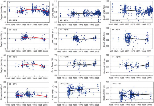
Fig. 7 Locations of O2 observations on the 26.3 σθ surface for the Gulf of Alaska north and west of Haida Gwaii (formerly the Queen Charlotte Islands) of the northwest coast of Canada. Symbol colours denote the decade of sampling. Grey and black lines are the 200 and 1500 m isobaths, respectively.
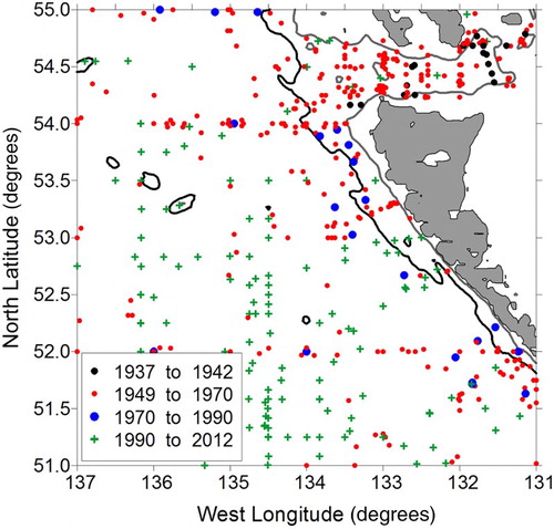
Fig. 8 Scatterplots of observations of O2 (left panel, μmol kg−1) and Θ (middle panel, °C) interpolated onto the 26.7 σθ surface, for the region to the north and west of Haida Gwaii (formerly the Queen Charlotte Islands) (51°–55°N, 131°–137°W). Depth of the 26.7 σθ surface is plotted in the right panel (m). Blue symbols represent individual observations. Red lines are significant quadratic polynomials of annual averages of O2. Black lines are best-fit quadratic polynomials to all observations of Θ and depth of the 26.7 σθ surface. Horizontal axes show the year of observation.
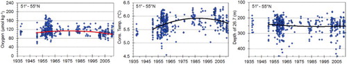
Fig. 9 Scatterplots of observations of O2 (μmol kg−1) versus year for three σθ surfaces: 26.3 (left), 26.5 (middle), and 26.9 (right), at locations along the continental slope from southern California to southern British Columbia and on the continental margin for the most northern region at 51°–55°N. Blue symbols represent individual observations. Red lines are significant quadratic polynomials of annual averages of these observations. Stations where no significant quadratic polynomials were found do not have red lines. Horizontal axes show the year of observation. Note the change in scale for O2 on the 26.9 σθ surface.
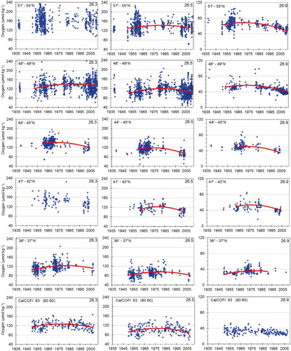
Fig. 10 Significant quadratic polynomials of annual averages at each station and region. Panels are for the following σθ surfaces: (a) 26.3, (b) 26.5; (c) 26.7; and (d) 26.9. (left panel) Northern stations from 36°N to 55°N and (right panel) CalCOFI stations.
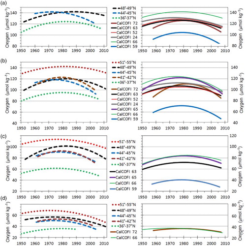
Fig. 11 Oxygen concentration interpolated onto three σθ surfaces at four stations along Line P: (a) OSP at 50.00°N, 145.00°W; (b) P20 at 49.57°N, 138.67°W; (c) P16 at 49.28°N, 134.67°W; and (d) P8 at 48.82°N, 128.67°W.
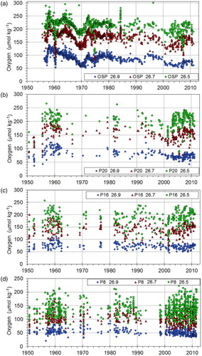
Table 2. Properties of the annual-average Line P time series of O2 on σθ surfaces. The 95% confidence limits are in parentheses. a lists the slope of the linear trend. Trends are not listed if the confidence limit exceeds the magnitude of the slope. b lists the amplitude and phase of the best-fit 18.61-year LNC to each time series for the 26.9 surface.
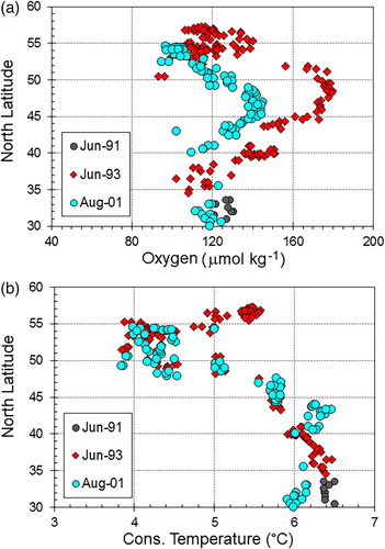
Fig. 12 (a) O2 and (b) Θ measured on WOCE line P1 along 47°N on the 26.7 σθ surface for each of three periods. Green lines in (a) indicate stations most likely to have been affected by a Haida Eddy.
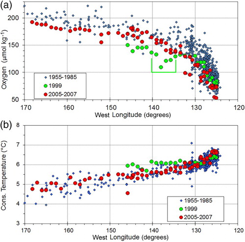
Fig. 13 Observations of (a) O2 and (b) Θ along a north–south section in the Northeast Pacific Ocean from 149.5°W to 161.2°W, excluding samples where bottom depth is less than 210 m. All values have been interpolated onto the 26.7 σθ surface. Colours denote time intervals as shown in the legends.
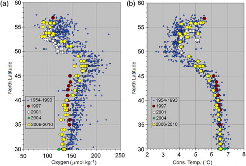
Table 3. Statistically significant differences in O2 (μmol kg−1) between the two periods 1954–1993 and 2006–2010 in the longitude range 149.5°–161.2°W. Columns for each period list the mean, the mean plus two standard errors, and the mean minus two standard errors. Numbers in bold indicate the lower limit for 1954–1993 and the upper limit for 2006–2010. The right column lists differences in the means.
Fig. 14 Observations of (a) O2 and (b) Θ on WOCE line P17 between 1991 and 2001 on the 26.7 σθ surface. The section extends northward along 135°W to 41°N, then heads towards 55°N, 159°W, as shown in f.