Hindcast of Water Level and Flow in the St. Lawrence River Over the 2005–2012 Period

Figures & data

Fig. 1 Model domain and position of water level gauges and flow sections from Lake St-Pierre to Québec.

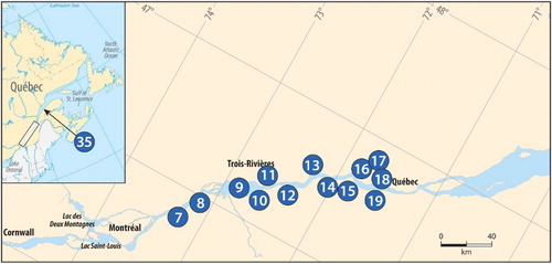
Fig. 2 Position of the water level gauges, flow sections, and meteorological stations in the downstream portion of the model domain.

Fig. 3 Position of the water level gauges around the Montréal Islands.

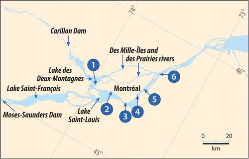
Fig. 4 Stage-discharge relationship at Pointe-Claire (Station 2) for the model upstream flow boundary conditions.

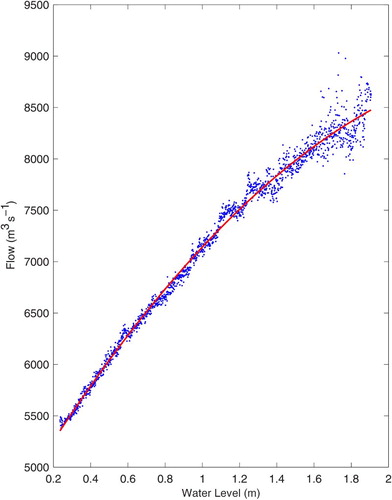
Fig. 5 Example of a storm surge observed at the Saint-Joseph-de-la-Rive (Station 34) water level gauge.

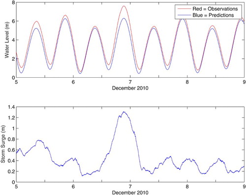
Fig. 6 Low-frequency oscillations at High Water and Low Water marks observed at Saint-Joseph-de-la-Rive water level gauge with a 30-day moving average filter on the residual (observations minus tidal predictions). The bottom curve is the daily average flow at the Vieux-Québec section (Station 21).

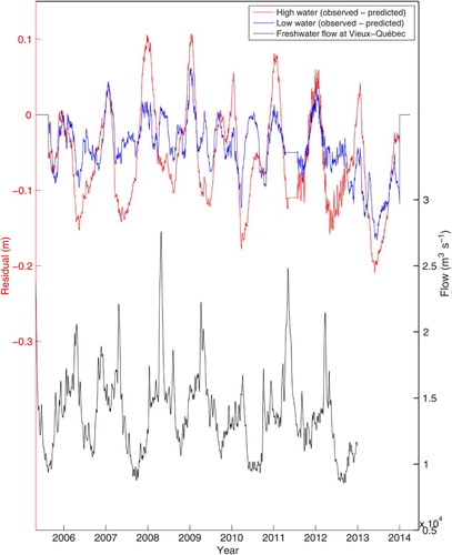
Fig. 7 Example of the water levels at the three downstream boundaries. The difference in amplitude and phase among the three is the result of the calibration process using the observed water levels at the tidal gauges upstream of the boundaries.

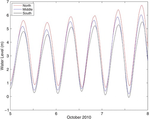
Fig. 8 Mean error, standard deviation, and γ² value of the model results for each tidal station. The tidal gauge number refers to the consecutive numbers in Table A2.

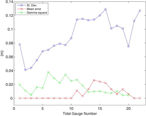
Fig. 9 Standard deviation of the model result errors at the downstream tidal stations. The tidal gauge number refers to the consecutive number of Table A2.

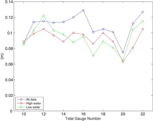
Fig. 10 Flows at the Vieux-Québec section (Station 21) derived from current measurements and from the model results, along with the ratio between the two values. The time on the abscissa is hours from 14:48 utc on 15 June 2009.

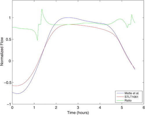
Table 1. The ratio of the model flow results to flows derived from ADCP measurements for the sections. Mean and standard deviation values are calculated excluding Station 27.

Station Number	Section	Mean Ratio
11	Trois-Rivières	0.84
12	Bécancour	0.87
13	Batiscan	0.85
15	Grondines	0.85
16	Deschambault	0.86
17	Portneuf	0.87
18	Neuville	0.87
19	Saint-Nicolas	0.82
21	Vieux-Québec	0.84
23	Lauzon	0.92
24	Beauport	0.86
26	Orléans Island South	0.89
27	Orléans Island North	0.63
	Mean value (without Station 27)	0.86
	St. Dev. (without Station 27)	0.02

Fig. 11 Daily flow values at the Vieux-Québec section (Station 21) for the years of the hindcast period 2005–2012. The flow on the ordinate is for 2005 data; 10,000 m³ s⁻¹ has been added consecutively to each following year for clarity.

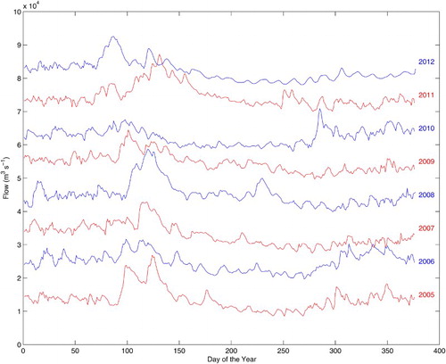
Fig. 12 Regression between the monthly-mean flows from the present model results with the monthly-mean flows using the Bourgault and Koutitonsky (1999) relationship.

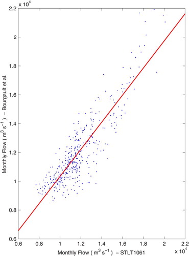
Fig. 13 Regression of daily flows between Bouchard and Morin (2000), based on upstream flows, and this study.

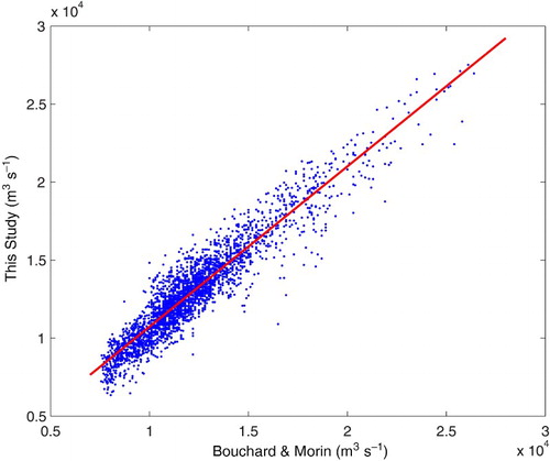
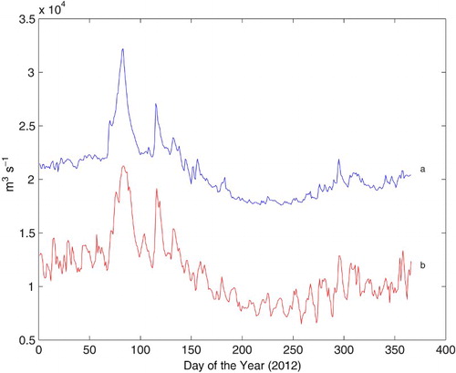
Fig. 14 Estimated flows from Bouchard and Morin (2000) for 2012 in a and this study in b; 10,000 m³ s⁻¹ has been added to the former for clarity.

Table A1. Geographical positions of the stations with observations of water level (WL), current (C), flow (F), and wind (W).

Station Number	Station Name	Latitude (°North)	Longitude (°West)	Qualifier
1	Sainte-Anne-de-Bellevue	45.405	−73.956	WL
2	Pointe-Claire	45.428	−73.821	WL
3	Lasalle	45.415	−73.623	WL, F
4	Montréal Harbour	45.503	−73.546	WL
5	Frontenac	45.528	−73.540	WL
6	Varennes	45.685	−73.454	WL
7	Contrecoeur	45.836	−73.288	WL
8	Sorel	46.054	−73.119	WL
9	Lake St-Pierre	46.191	−72.894	WL
10	Port St-François	46.274	−72.621	WL
11	Trois-Rivières	46.335	−72.531	WL, C
12	Bécancour	46.410	−72.386	WL, C
13	Batiscan	46.497	−72.232	WL, C
14	Deschaillons	46.565	−72.106	WL
15	Grondines	46.575	−72.031	C
16	Deschambault	46.652	−71.907	C
17	Portneuf	46.678	−71.875	WL, C
18	Neuville	46.680	−71.563	WL, C
19	St-Nicolas	46.723	−71.382	C
20	Québec's Bridge	46.746	−71.287	WL
21	Vieux-Québec	46.811	−71.195	WL, C
22	Québec City Jean Lesage International Airport	46.800	−71.349	W
23	Lauzon	46.842	−71.164	WL, C
24	Beauport	46.855	−71.154	C
25	St-Laurent	46.854	−71.002	WL
26	Orléans I. South	46.904	−70.886	C
27	Orléans I. North	46.958	−71.012	C
28	Saint-François	46.994	−70.802	WL, W
29	Banc-Cap-Brûlé	47.093	−70.717	WL
30	Grosse-Île	47.020	−70.671	WL
31	Rocher Neptune	47.174	−70.639	WL
32	Île-aux-Grues	47.055	−70.532	WL,W
33	Saint-Jean-Port-Joli	47.216	−70.275	WL
34	St-Joseph-de-la-Rive	47.437	−70.363	WL
35	Rimouski	48.480	−68.510	WL

Table A2. List of water level stations and length of the water level time series. The Consecutive Number is the number used in Figs 8 and 9.

Consecutive Number	Station Number	Water Level Gauge	Years
	1	Sainte-Anne-de-Bellevue	2005–2013
	2	Pointe-Claire	2005–2013
	3	Lasalle	2005–2013
1	4	Montréal Harbour	2005–2013
2	5	Frontenac	2005–2013
3	6	Varennes	2005–2013
4	7	Contrecoeur	2005–2013
5	8	Sorel	2005–2013
6	9	Lake St-Pierre	2005–2013
7	10	Port St-François	2005–2013
8	11	Trois-Rivières	2005–2013
9	12	Bécancour	2005–2013
10	13	Batiscan	2005–2013
11	14	Deschaillons	2005–2013
12	17	Portneuf	2005–2013
13	18	Neuville	2005–2013
14	20	Québec's Bridge	Summer 2012
15	21	Vieux-Québec	2012–2013
16	23	Lauzon	2005–2012
17	25	Saint-Laurent	Summer 2012
18	28	Saint-François	2005–2013
19	29	Banc-Cap-Brûlé	Summers 2005–2013
21	30	Grosse-Île	Summer 2010
20	31	Rocher Neptune	Summers 2005–2013
22	32	Île-aux-Grues	Summer 2010
	33	Saint-Jean-Port-Joli	1974
	34	St-Joseph-de-la-Rive	2005–2013
	35	Rimouski	2005–2013

Table A3. List of the sections with current measurements.

Station Number	Section	Date	Observation (Hours)	Error in the Flow (%)
11	Trois-Rivières	18 June 2009	0.8	1.7
12	Bécancour	18 June 2009	5.0	2.1
13	Batiscan	23 June 2009	7.6	7.3
15	Grondines	19 June 2009	8.9	1.8
16	Deschambault	20 August 2009	10.1	6.3
17	Portneuf	26 June 2009	6.7	4.5
18	Neuville	25 June 2009	9.1	2.3
19	Saint-Nicolas	21 August 2009	8.8	2.2
21	Vieux-Québec	15 June 2009	11.3	4.7
23	Lauzon	24 June 2009	11.4	3.1
24	Beauport	24 June 2009	10.7	14.7
26	Orléans I. South	24 August 2009	7.6	2.1
27	Orléans I. North	25 August 2009	8.7	5.4

Bourgault, D., & Koutitonsky, V. G. (1999). Real-time monitoring of the freshwater discharge at the head of the St. Lawrence Estuary. Atmosphere-Ocean, 37, 203–220. doi: 10.1080/07055900.1999.9649626

 Web of Science ®Google Scholar

Bouchard, A., & Morin, J. (2000). Reconstitution des débits du fleuve Saint-Laurent entre 1932 et 1998. Rapport Technique RT-101, Environnement Canada, Sainte-Foy.

 Google Scholar