Seasonal Cycles, Hypoxia, and Renewal in a Coastal Fjord (Barkley Sound, British Columbia)

Figures & data

Fig. 1 Barkley Sound, British Columbia. Location of main map is shown by hatched area in inset map. A contour line is drawn at 50 m, and areas deeper than 150 m (occuring in Effingham and Alberni Inlets) are hatched. Hydrographic stations are marked with red stars, the La Perouse weather buoy with a black star, river flow gauges with red circles, and the Bamfield tide station with a red square.

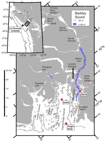
Fig. 2 Climatological average daily flows in the Somass and Sarita Rivers. Shaded area represents ± 1 standard deviation of Somass River flow over the years 1958–2003. Also shown is the Somass flow in 1996 and the mean Somass flow estimated by scaling the mean Sproat River flow using Eq. (1).

Fig. 3 Sarita station profiles in Trevor Channel during (left) winter and (right) summer.

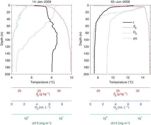
Fig. 4 (a) Temperatures at 2 m for the Sarita and Swale stations. (b) The annual signal in near-surface temperature. Times during which deep water density (below 140 m) is increasing are shaded in grey.

Fig. 5 (a) Salinities at 2 m for the Sarita and Swale stations. (b) The annual signal in near-surface salinity. Times during which deep water density (below 140 m) is increasing are shaded in grey.

Fig. 6 Seasonal cycles of (a) temperature, (b) salinity, (c) density, and (d) dissolved oxygen for Swale station in Eagle Channel. (e) to (h) As in (a) to (d) but for Sarita station in Trevor Channel. Time interval plotted is from June 2008 to August 2009. The white lines in (d) and (h) mark the hypoxic limit (1.4 mL L⁻¹).

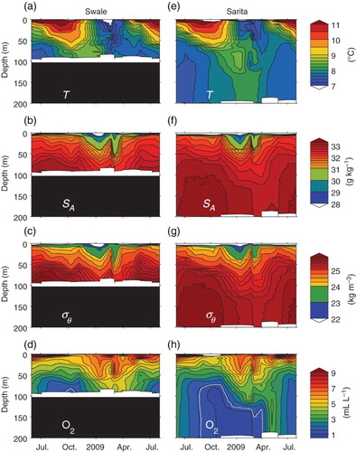
Fig. 7 (a) FWE and (b) depth-integrated chlorophyll biomass. The mean summer conditions (between the spring increase and the fall decrease in chlorophyll biomass) are shown as horizontal bars. Times during which deep water density is increasing are shaded in grey.

Fig. 8 Correlations between (a) time of the spring increase and summer FWE; (b) mean summer biomass and mean summer FWE; (c) mean summer biomass and the timing of the spring increase.

Fig. 9 (a) Density of the deep and intermediate waters. (b) Alongshore winds at La Perouse and sea level at Bamfield (low-pass filtered with a two-week cutoff). Times during which deep water density is increasing are shaded in grey.

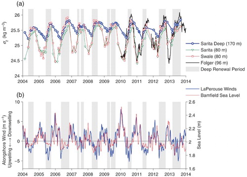
Fig. 10 (a) Temperatures and (b) dissolved oxygen concentrations in the deep and intermediate waters. Times during which deep water density is increasing are shaded in grey.

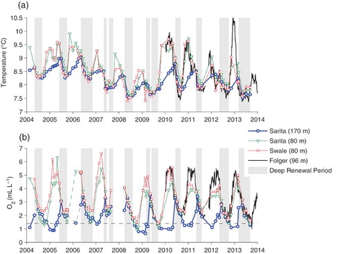
Fig. 11 Sections along Trevor Channel and Alberni Inlet in June 2007 and February 2009. (a) Summer temperature, (b) winter temperature, (c) summer salinity, (d) winter salinity, (e) summer dissolved oxygen, and (f) winter dissolved oxygen. The white line marks the hypoxic limit in winter. Distances are inshore of the coast. The Sarita station is at kilometre 27.

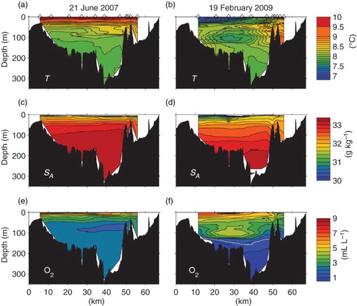
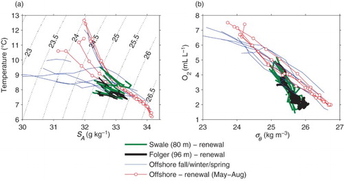
Fig. 12 (a) Correlations between climatological temperature and salinity for offshore waters. Each curve is the climatological mean for a particular month; summer and winter curves are shown differently. Also shown are curves, one per year for the deep renewal period only, showing the T/S characteristics of inflowing water at Swale and Folger stations. (b) Correlations between climatological oxygen and density for offshore waters. Although the depth of isopycnals changes dramatically over the year, the concentrations of oxygen at a particular isopycnal are relatively constant. Also shown are curves, one per year for the deep renewal periods only, showing the oxygen/density characteristics of inflowing water at Swale and Folger stations. Bottom waters at the beginning of the renewal period are lightest, and those at the end are most dense.