Dynamical Downscaling of Temperature and Precipitation Extremes in China under Current and Future Climates

Figures & data

Fig. 1 The WRF model domain and topography (m). The eight sub-regions used in the analysis are identified (1: western part of Northwest China; 2: eastern part of Northwest China; 3: North China; 4: Northeast China; 5: Tibetan Plateau; 6: Southwest China; 7: Yangtze River Valley (middle and lower); 8: South China (includes Hainan and Taiwan islands)).

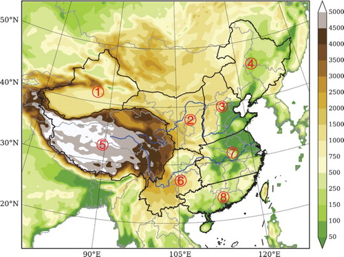
Table 1. Definitions and units of the 12 climate extreme indices used in this study (see http://www.climdex.org/indices.html).

	Index	Definitions	Units
Temperature indices	Tx90p	Percentage of days when the daily maximum temperature is higher than the 90th percentile of daily maximum temperature	%
	Tx10p	Percentage of days when the daily maximum temperature is lower than the 10th percentile of daily maximum temperature	%
	Tn90p	Percentage of days when the daily minimum temperature is higher than the 90th percentile of daily minimum temperature	%
	Tn10p	Percentage of days when the daily minimum temperature is lower than the 10th percentile of daily minimum temperature	%
	FD	Number of days when the daily minimum temperature is lower than 0°C	days
	SU	Number of days when the daily maximum temperature is higher than 25°C	days
	ID	Number of days when the daily maximum temperature is lower than 0°C	days
	TR	Number of days when the daily minimum temperature is higher than 20°C	days
Precipitation indices	R95p	Number of days with daily precipitation larger than 95th percentile	days
	Rx5day	Maximum five-day precipitation amount	mm
	R10mm	Number of days when the daily precipitation is larger than or equal to 10 mm	days
	CDD	Maximum number of consecutive days when precipitation is less than 1 mm	days

Fig. 2 Spatial distribution of seasonal mean surface air temperature (°C) averaged during the 1996–2005 period as observed (OBS) and as simulated by CCSM4 and downscaled by WRF: (a) OBS (MAM), (b) CCSM4 (MAM), (c) WRF (MAM), (d) OBS (JJA), (e) CCSM4 (JJA), (f) WRF (JJA), (g) OBS (SON), (h) CCSM4 (SON), (i) WRF (SON), (j) OBS (DJF), (k) CCSM4 (DJF), and (l) WRF (DJF), where MAM is March, April, and May; JJA is June, July, and August; SON is September, October, and November; and DJF is December, January, and February.

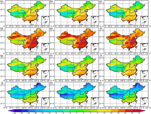
Fig. 3 Spatial distribution of seasonal mean surface air temperature bias (°C) averaged during the 1996–2005 period as simulated by CCSM4 and downscaled by WRF.

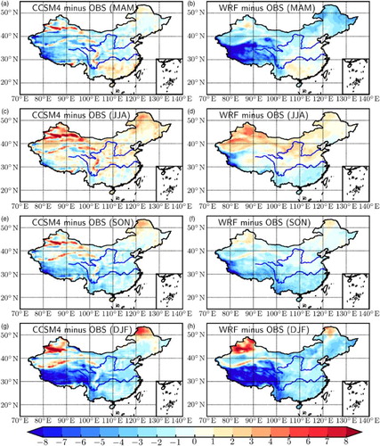
Fig. 4 Spatial distribution of seasonal mean daily precipitation (mm d⁻¹) averaged during the 1996–2005 period as observed (OBS) and simulated by CCSM4 and downscaled by WRF: (a) OBS (MAM), (b) CCSM4 (MAM), (c) WRF (MAM), (d) OBS (JJA), (e) CCSM4 (JJA), (f) WRF (JJA), (g) OBS (SON), (h) CCSM4 (SON), (i) WRF (SON), (j) OBS (DJF), (k) CCSM4 (DJF), and (l) WRF (DJF).

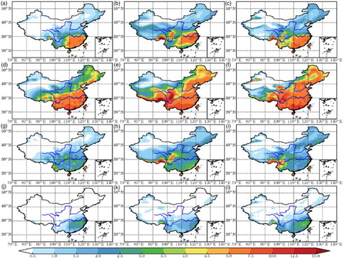
Fig. 5 Annual cycles of precipitation bias ratios (relative to observations) during the 1996–2005 period simulated by CCSM4 and downscaled by WRF averaged over the eight sub-regions in Fig. 1.

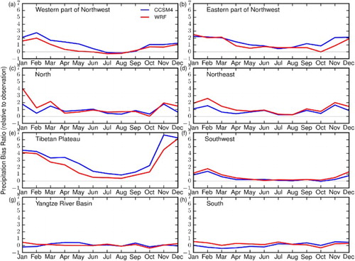
Table 2. Climatological seasonal spatial pattern correlation coefficients between observations and CCSM4, observations and WRF, CCSM4 and WRF for precipitation and surface air temperature during the 1996–2005 period.

	OBS and CCSM4	OBS and WRF	CCSM4 and WRF
Precipitation
Winter	0.76	0.84	0.88
Spring	0.72	0.86	0.79
Summer	0.65	0.81	0.80
Autumn	0.60	0.65	0.81
Temperature
Winter	0.94	0.95	0.96
Spring	0.95	0.98	0.96
Summer	0.95	0.98	0.96
Autumn	0.96	0.98	0.96

Fig. 6 Spatial distribution of projected seasonal (MAM, JJA, SON, and DJF) mean surface air temperature differences (°C) (between the 2046–2055 and 1996–2005 averages) under RCP4.5 and RCP8.5 simulated by CCSM4 and downscaled by WRF.

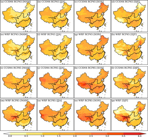
Fig. 7 Spatial distribution of projected seasonal (MAM, JJA, SON, and DJF) mean precipitation change (%) (differences between the averages during the 2046–2055 period and the 1996–2005 period relative to averages during the 1996–2005 period) under RCP4.5 and RCP8.5 simulated by CCSM4 and downscaled by WRF.

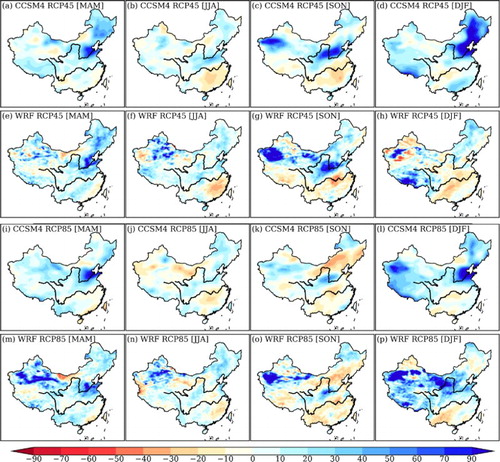
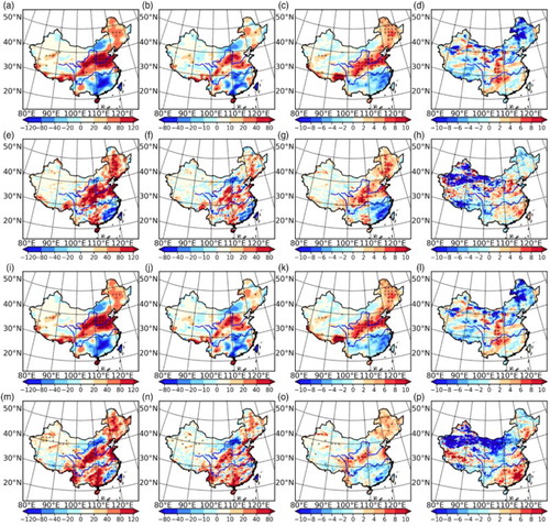
Fig. 8 Spatial distributions of future changes of annual (a), (e), (i), and (m) TX90p (%); (b), (f), (j), and (n) TX10p (%); (c), (g), (k), and (o) TN90p (%); and (d), (h), (l), and (p) TN10p (%) under the (a)–(h) RCP4.5 and (i)–(p) RCP8.5 emission scenarios for the 2046–2055 period relative to the historical run for the 1996–2005 period; crosses indicate changes significant at the p = 0.05 level based on a Student’s t-test. CCSM4 results are in the 1st (a)–(d) and 3rd (i)–(l) rows. WRF results are in the 2nd (e)–(h) and 4th (m)–(p) rows.

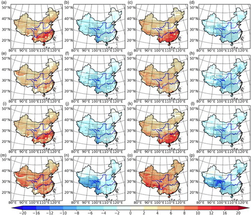
Fig. 9 Spatial distributions of future changes in annual (a), (e), (i), and (m) FD (days); (b), (f), (j), and (n) SU (days); (c), (g), (k), and (o) ID (days); and (d), (h), (l), and (p) TR (days) under the (a)–(h) RCP4.5 and (l)–(p) RCP8.5 emission scenarios for the 2046–2055 period relative to the historical run for the 1996–2005 period; crosses indicate changes significant at the p = 0.05 level based on a Student’s t-test. CCSM4 results are in the 1st (a)–(d) and 3rd (i)–(l) rows. WRF results are in the 2nd (e)–(h) and 4th (m)–(p) rows.

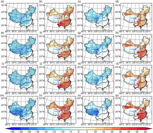
Table 3. Future changes in annual mean temperature climate extreme indices (Tx90p, Tx10p, Tn90p, and Tn10p) under RCP4.5 and RCP8.5 emission scenarios for the 2046–2055 period relative to the 1996–2005 period for eight regions of China (see Fig. 1).

Sub-regions	Temperature Climate Extreme Indices
	RCP4.5 minus HIS				RCP8.5 minus HIS
	Tx90p (%)	Tx10p (%)	Tn90p (%)	Tn10p (%)	Tx90p (%)	Tx10p (%)	Tn90p (%)	Tn10p (%)
1	4.46	−1.69	4.77	−1.07	6.68	−0.93	6.84	−0.61
2	3.88	−2.71	4.33	−2.25	6.92	−1.17	6.40	−1.06
3	4.36	−2.73	4.42	−2.64	6.44	−2.00	6.15	−1.61
4	2.97	−1.85	3.37	−2.79	4.66	−2.10	5.32	−2.86
5	3.27	−4.05	4.96	−3.89	5.78	−7.16	7.91	−6.94
6	3.66	−4.52	4.18	−4.31	6.07	−4.67	6.73	−5.04
7	5.36	−3.49	3.18	−2.78	7.26	−2.48	4.87	−2.43
8	4.30	−2.94	3.77	−2.88	6.37	−2.48	6.06	−2.95

Table 4. Future changes in annual mean temperature climate extreme indices (FD, SU, ID, and TR) under RCP4.5 and RCP8.5 emission scenarios for the 2046–2055 period relative to the 1996–2005 period for eight regions of China (see Fig. 1).

Sub-regions	Temperature Climate Extreme Indices
	RCP4.5-HIS				RCP8.5-HIS
	FD (days)	SU (days)	ID (days)	TR (days)	FD (days)	SU (days)	ID (days)	TR (days)
1	−13.3	8.9	−9.8	14.5	−12.8	14.1	−6.7	20.3
2	−14.6	10.7	−11.1	9.2	−12.2	20.6	−4.4	14.2
3	−14.7	11.5	−10.4	10.4	−12.6	20.7	−6.0	13.5
4	−11.7	10.6	−11.4	3.7	−13.8	15.7	−11.9	6.8
5	−17.1	0.7	−15.4	0.2	−26.7	1.3	−24.7	0.3
6	−12.3	18.2	−1.1	11.6	−13.5	25.9	−0.1	16.5
7	−10.3	16.5	−1.6	19.9	−9.2	21.8	0.5	25.2
8	−3.2	18.8	0.0	21.8	−2.7	22.2	0.2	31.0

Fig. 10 Spatial distributions of future changes in annual (a), (e), (i), and (m) R95p (days); (b), (f), (j), and (n) Rx5day (mm); (c), (g), (k), and (o) R10mm (days); and (d), (h), (l), and (p) CDD (days) under the (a)–(h) RCP4.5 and (i)–(p) RCP8.5 emission scenarios for the 2046–2055 period relative to the historical run for the 1996–2005 period; crosses indicate changes significant at the p = 0.05 level based on a Student’s t-test. CCSM4 results are in the 1st (a)–(d) and 3rd (i)–(l) rows. WRF results are in 2nd (e)–(h) and 4th (m)–(p) rows.

TABLE 5. Future changes in annual mean precipitation climate extreme indices under RCP4.5 and RCP8.5 emission scenarios for the 2046–2055 period relative to the 1996–2005 period for eight regions of China (see Fig. 1).

Sub-regions	Precipitation Climate Extreme Indices
	RCP4.5-HIS				RCP8.5-HIS
	R95p (days)	Rx5day (mm)	R10mm (days)	CDD (days)	R95p (days)	Rx5day (mm)	R10mm (days)	CDD (days)
1	8.4	2.8	0.6	−7.2	14.4	3.5	0.8	−11.9
2	37.0	8.6	2.1	−2.9	23.4	5.6	1.0	−10.5
3	61.6	5.3	3.8	2.2	36.1	4.1	1.6	−2.3
4	46.5	10.7	3.5	−1.0	48.2	13.1	3.3	0.5
5	16.0	4.9	1.1	−1.2	16.8	5.6	1.1	0.2
6	32.1	10.5	1.6	0.0	51.2	19.6	0.3	−0.1
7	17.1	13.0	−1.7	1.8	40.5	12.6	−0.6	2.8
8	2.3	−2.2	−1.7	1.3	48.0	29.7	−1.5	4.4