The Ocean Circulation of Chatham Sound, British Columbia, Canada: Results From Numerical Modelling Studies Using Historical Datasets

Figures & data

Fig. 1 Location of Chatham Sound (marked by red box) based on gridded bathymetry data from GEBCO (2014).

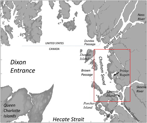
Fig. 2 Map of water depths in Chatham Sound (metres below chart datum, CHS). Predicted water levels are located at sites (Table 1) in red. Current meter sites (RUP2 and CP01S, see Table 2) are marked as red dots. Wind stations (data presented in Fig. 3) are in orange. Grey lines outline the model domain.

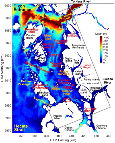
Table 1. Largest predicted tidal heights based on measured values in Chatham Sound.

Station	Record Duration (years)	Peak Water Level (m)	Maximum Tidal Range (m)
Lawyer Islands	0.1	3.53	7.04
Qlawdzeet Anchorage	0.2	3.27	6.62
Moffatt Islands	0.2	3.20	6.17
Brundige Inlet	0.1	3.15	6.32
Prince Rupert	104.7	3.64	7.41
Port Simpson	87.6	3.44	7.07

Table 2. Current meter data used for model verification.

Site	Location	Year	Season	Current Bin Depth (m)	Water Depth (m)
RUP2	54.20°N 130.36°W	1993	summer	17	37
CP01S	54.42°N 130.66°W	1991/92	winter	14	69

Fig. 3 Compass rose plots for bivariate wind speed and direction distributions measured at (a) Lucy Island, (b) Grey Islet, (c) Prince Rupert Airport, and (d) Holland Rock. The wind datasets were obtained from the Meteorological Service of Canada, Environment and Climate Change Canada.

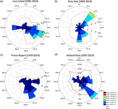
Fig. 4 Daily discharge values of (a) the Skeena River measured at Usk and (b) the Nass River (derived from Water Survey of Canada datasets).

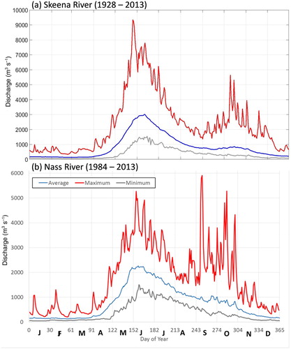
Fig. 5 Enhanced Landsat 8 satellite image for 28 August 2013 (left panel, ebb flow, 665 m³ s⁻¹ river discharge) and 5 April 2015 (right panel, flood flow, 200 m³ s⁻¹ river discharge) under low to moderate discharges from the Skeena River.

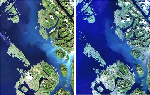
Fig. 6 Historical CTD and bottle data for BC coastal waters. Sites are grouped as southern (blue box), western (black box), and northern (red box) Chatham Sound. Data obtained in the earlier measurement period are from reversing bottle measurements, while most data in the latter period are obtained using CTD instruments.

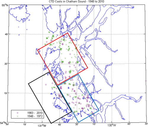
Fig. 7 Seasonal temperature and salinity plots based on CTD and bottle observations in (a) southern, (b) western, and (c) northern Chatham Sound as shown in Fig. 6.

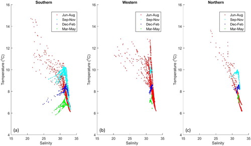
Fig. 8 Model-generated water levels (MOD, blue solid lines) in the summer run (1993) at the two sites marked in Fig. 2, with comparisons to observational data (OBS, red dashed lines) from the predicted tidal elevations (PTE) derived from CHS tidal datasets and observed water levels at the Prince Rupert tidal gauge (TG). The water levels are plotted relative to chart datum (0).

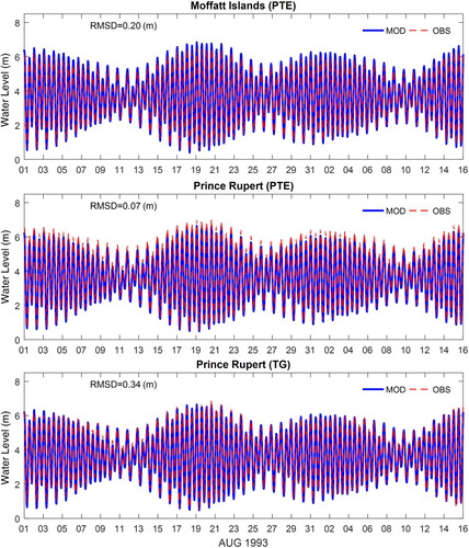
Fig. 9 Model-generated water levels (MOD, blue solid lines) in the winter run (1991/92) at the two sites marked in Fig. 2, with comparisons to observational data (OBS, red dashed lines) from the predicted tidal elevations (PTE) derived from CHS tidal datasets and observed water levels at the Prince Rupert tidal gauge (TG). The water levels are plotted relative to chart datum (0).

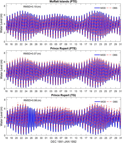
Fig. 10 (a) Model-generated hourly averaged current speed in August–September 1993 (blue line) at a depth of 17 m at RUP2 marked in Fig. 2, with comparisons to observations (red line). (b) Model-generated current vectors (blue dots) are compared with observations (red crosses). The numbers on the outer ring represent current directions in degrees clockwise from true north while the row of numbers on the smaller to larger circles are current speeds (cm s⁻¹). (c) Current speed histogram for model results (blue dashed line) and observations (red line).

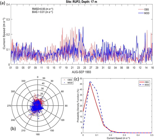
Fig. 11 (a) Model-generated hourly averaged current speed from December 1991 to January 1992 (blue line) at a depth of 14 m at CP01S marked in Fig. 2, with comparisons to observation (red line). (b) Model-generated current vectors (blue dots) are compared with observations (red crosses). The numbers on the outer ring represent current directions in degrees clockwise from true north, while the row of numbers on the smaller to larger circles are current speeds (cm s⁻¹). (c) Current speed histogram for model results (blue dashed line) and observations (red line).

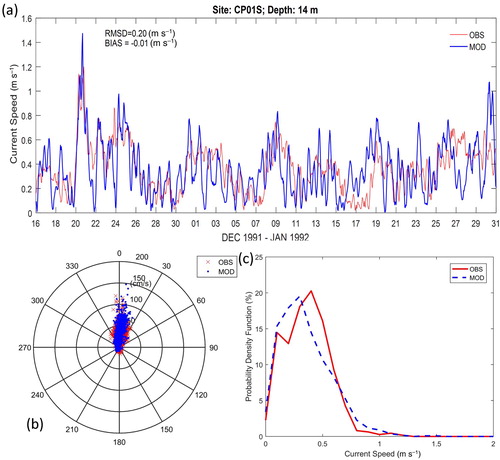
Fig. 12 Hourly wind vectors (direction from) measured at Lucy Island in 2003.

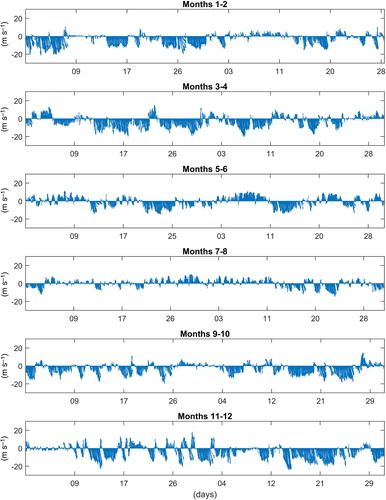
Fig. 13 Daily discharge values of the Skeena and Nass Rivers in 2003.

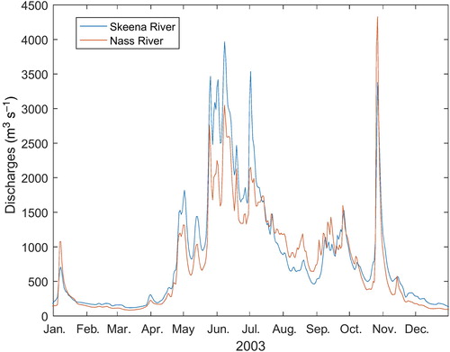
Fig. 14 M₂ tidal ellipse plots (sub-sampled every seven model grids) of (a) surface (uppermost model layer), (b) mid-depth (middle model layer), and (c) near-bottom (deepest model layer) currents over Chatham Sound, during the one-year model simulation. (d) Barotropic M₂ model current tidal ellipses adapted from Fig. 7 in Foreman et al. (1993). Contours are water depth (m).

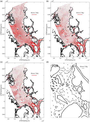
Fig. 15 Temporally averaged total current vectors at the surface in (a) summer (June–August) and (b) winter (December–February) in southern Chatham Sound (sub-sampled every five model grids). Temporally averaged surface salinities for (c) June–August and (d) December–February.

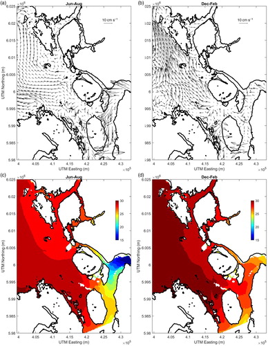
Fig. 16 Seasonal mean residual flow anomalies (annual mean values and tidal flow have been removed) at the surface in (a) summer (June–August) and (b) winter (December–February) in southern Chatham Sound (sub-sampled every five model grids). (c) Distribution of correlation coefficients between daily mean surface current speeds and wind speeds observed at Lucy Island. (d) Distribution of correlation coefficients between daily mean surface current speeds and Skeena River discharges measured at Usk (shifted 20 days later). Water depths (m) relative to chart datum are denoted by the numbered grey contours.

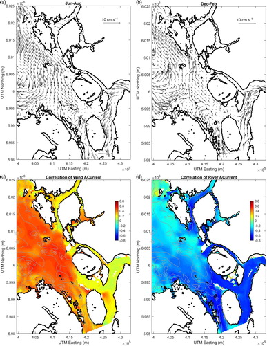
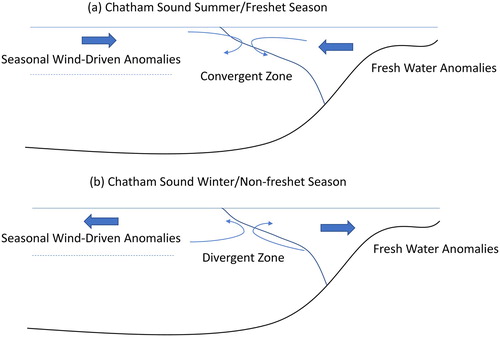
Fig. 17 Schematic diagrams of two-layer flow anomalies in (a) the summer or freshet and (b) the winter or non-freshet season in southern Chatham Sound.

GEBCO. (2014). Gridded bathymetry data. Retrieved from the website of the British Oceanographic Data Centre: https://www.gebco.net/data_and_products/gridded_bathymetry_data

 Google Scholar

Foreman, M. G. G., Henry, R. F., Walters, R. A., & Ballantyne, V. A. (1993). A finite element model for tides and resonance along the north coast of British Columbia. Journal of Geophysical Research: Oceans, 98(C2), 2509–2531. doi: 10.1029/92JC02470

 Web of Science ®Google Scholar