Wind Waves in the Strait of Georgia

Figures & data

Fig. 1 (a) Location of the Strait of Georgia and WW3 mode domain. (b) Strait of Georgia. Shading indicates coastline, 500 m, and 1000 m elevation contours.

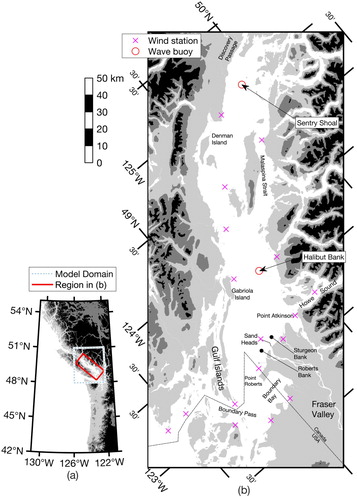
Fig. 2 Wave spectra from (a) Halibut Bank and (b) Sentry Shoal, plotted on a log/log scale. Curves are observations taken every 100 h over the period of data availability. The dashed red line shows the universal high-frequency tail of the Pierson–Moskowitz spectrum, which is commonly used as a standard description of saturated wind-waves. The blue line shows an $f^{-4}$ dependence with an arbitrary height scaling.

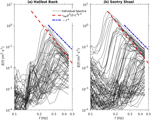
Fig. 3 Comparison of the significant wave height $H_s$ from the wave model and the buoy observations January 2018. Both data are at the same hourly resolution. The grey lines depict the model wind speed $U_{10}$. Top: results for Halibut Bank in the central Strait of Georgia. Bottom: results for Sentry Shoal in the northern Strait of Georgia.

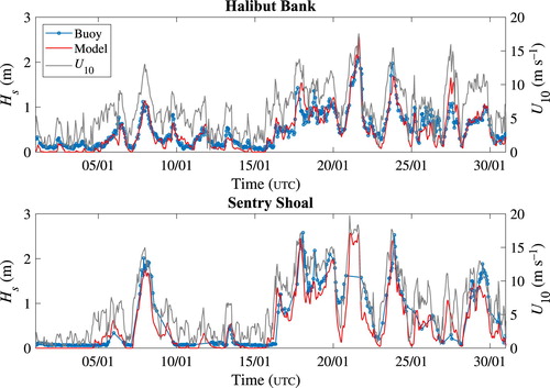
Fig. 4 Comparison of wave model output and buoy observations for the period 1 April 2017 to 22 November 2018. (a) and (b) Significant wave height $H_s$; (c) and (d) mean wave period $T_m$; (e) and (f) wind speed $U_{10}$. Bias b and scatter index SI are given on each panel. Colour indicates data density as counts per cell, given by the colour bars.

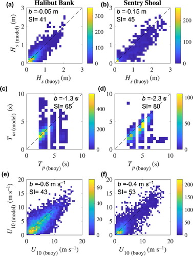
Fig. 5 Discrepancy of significant wave height $H_s$ between model and observations as a function of wind speed $U_{10}$ discrepancies. Colour indicates data density as counts per cell, given by the colour bars.

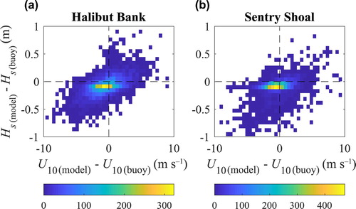
Fig. 6 Wind roses for hourly winds during a 2-year period starting 12 April 2017. The background circles in each rose are 2.5% and 5%.

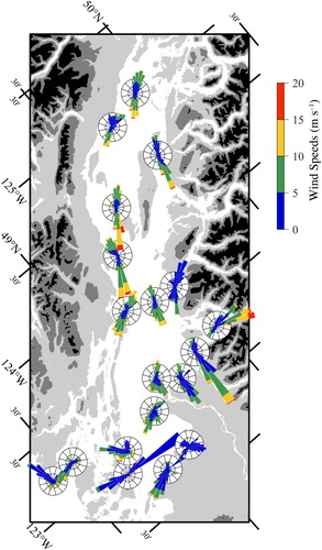
Table 1. Percentage of time in different wind speed and direction conditions at Halibut Bank from April 2017 to April 2019 from the ECCC model output and buoy observations (in parentheses), respectively.

	SE (${90}^{\circ }-{150}^{\circ }$)	SW (${150}^{\circ }-{270}^{\circ }$)	NW (${270}^{\circ }-{330}^{\circ }$)	NE (${330}^{\circ }-{90}^{\circ }$)	Total
(m s^−1)	(%)	(%)	(%)	(%)	(%)
$0-5$	17.7 (13.3)	11.7 (12.0)	21.5 (12.5)	6.2 (12.2)	57.1 (50.0)
$5-10$	15.5 (21.5)	2.2 (5.0)	19.0 (14.8)	0.8 (2.1)	37.2 (43.4)
$>10$	3.6 (4.8)	0.3 (0.6)	1.6 (1.1)	0.2 (0.1)	5.7 (6.6)
Totals	36.5 (39.6)	14.2 (17.6)	42.1 (24.4)	7.2 (14.4)	100 (100)

Fig. 7 Average wind speed in the Strait of Georgia, as a function of wind direction (columns) and wind speed (rows) at Halibut Bank [(a)–(c), (e)–(g)], and Howe Sound [(d) and (h)]. Top row: moderate Halibut Bank or Howe Sound winds ($5\mathrm{m}{\mathrm{s}}^{-1}\le U_{10}\le 10\mathrm{m}{\mathrm{s}}^{-1}$); bottom row: high Halibut Bank or Howe Sound winds ($U_{10}>10\mathrm{m}{\mathrm{s}}^{-1}$). The red arrows indicate the range of Halibut Bank wind directions in each average. The occurrence rate of the given wind speed and wind direction range at Halibut Bank is stated in the centre left of each of the three leftmost panels. Black arrows are wind vectors, subsampled by a factor of six from the HRDPS model grid.

Fig. 8 Significant wave height $H_s$ in the Strait of Georgia for low wind speeds ($U_{10}<5\mathrm{m}{\mathrm{s}}^{-1}$) at Halibut Bank as a function of wind direction (columns). (a)–(d): mean $H_s$, (e)–(h) 99th percentile of $H_s$. The red arrows indicate the range of wind directions. The occurrence rate of the given wind speed and wind direction range is stated on the centre left of each panel.

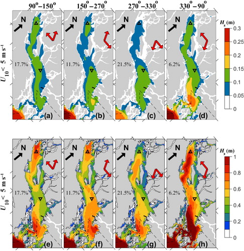
Fig. 9 As in Fig. 7, but showing mean significant wave height $H_s$ in the Strait of Georgia.

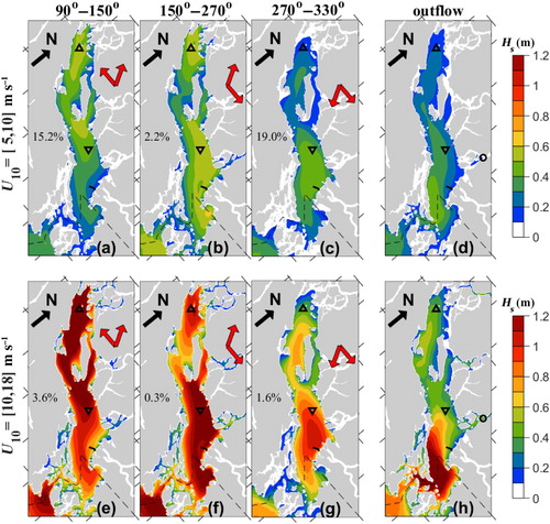
Fig. 10 As in Fig. 7, but showing average of the mean wave period $T_m$ in the Strait of Georgia.

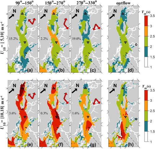
Fig. 11 As in Fig. 7, but showing 99th percentile of significant wave height $H_s$ in the Strait of Georgia.

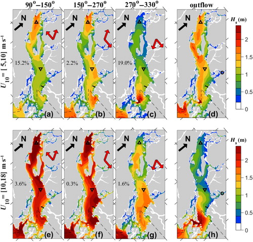
Fig. 12 As in Fig. 7, but showing the average of the mean whitecap coverage γ in the Strait of Georgia.

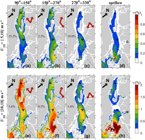
Fig. 13 As in Fig. 7, but showing the average of the mean Stokes drift (wave-induced current) $u_{\mathrm{S}\mathrm{t}}$ in the Strait of Georgia.

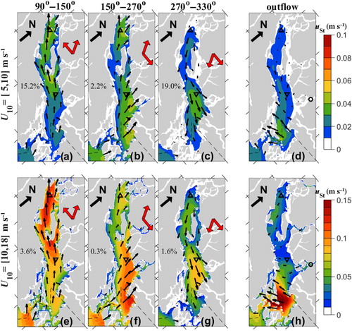
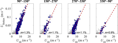
Fig. 14 Calculated Stokes drift versus wind speed at Halibut Bank: hourly data and least squares linear fit. Data are divided into $U_{10}\ge 5\mathrm{m}{\mathrm{s}}^{-1}$ (blue crosses, red line) with linear slope m given on each panel, and $U_{10}<5\mathrm{m}{\mathrm{s}}^{-1}$ (grey circles, grey line).

Table 2. Linear regression of modelled Stokes drift as a function of wind speed (Eq. (10(10) $u_{\mathrm{S}\mathrm{t}\mathrm{o}\mathrm{k}\mathrm{e}\mathrm{s}}\approx s\times U_{10}-u_{\mathrm{o}\mathrm{f}\mathrm{f}};s=0.011,u_{\mathrm{o}\mathrm{f}\mathrm{f}}=0.04\mathrm{m}{\mathrm{s}}^{-1}$(10) )) for different wind directions.

	SE (${90}^{\circ }-{150}^{\circ }$)	SW (${150}^{\circ }-{270}^{\circ }$)	NW (${270}^{\circ }-{330}^{\circ }$)	NE (${330}^{\circ }-{90}^{\circ }$)
s	0.0129	0.0111	0.0109	0.0086
$u_{\mathrm{o}\mathrm{f}\mathrm{f}}$ ($\mathrm{m}{\mathrm{s}}^{-1}$)	0.0583	0.0410	0.0441	0.0333