Cloud Microphysics in Global Cloud Resolving Models

Figures & data

Table 1. List of acronyms of models, satellites, and instruments.

Acronym	Long name
AMSR-E	Advanced Microwave Scanning Radiometer-EOS
AROME	Applications of Research to Operations at Mesoscale
ARPEGE-NH	Action de Recherche Petite Echelle Grande Echelle-NonHydrostatic version
CALIPSO/CALIOP	Cloud-Aerosol Lidar and Infrared Pathfinder Satellite Observations/Cloud-Aerosol LIdar with Orthogonal Polarization
CAM	Community Atmosphere Model
COSP	The cloud feedback model intercomparison project Observation Simulator Package
CPR	Cloud Profiling Radar
CRTM	Community Radiative Transfer Model
DFSM	Double Fourier Series Model
EarthCARE	Earth Clouds, Aerosols and Radiation Explorer
ECHAM	European Centre Hamburg model
ECSIM	EarthCARE Simulator
FV3	Finite-Volume Cubed-Sphere Dynamical Core
GCOM-C/SGLI	Global Change Observation Mission-Climate/ Second-generation Global Imager
GEOS	Goddard Earth Observing System
GOES	Geostationary Operational Environmental Satellite
GPM/DPR/GMI	Global Precipitation Measurement mission/Dual-frequency Precipitation Radar/GPM Microwave Imager
GRIST	Global-to-Regional Integrated forecast SysTem
ICON	ICOsahedral Non-hydrostatic atmospheric model
IFS	Integrated Forecasting System
MIROC	Model for Interdisciplinary Research on Climate
MODIS	Moderate Resolution Imaging Spectroradiometer
MSSG	Multi-Scale Simulator for the Geoenvironment
MPAS	Model for Prediction Across Scales
MTSAT	Multi-functional Transport Satellite
NICAM	Nonhydrostatic ICosahedral Atmospheric Model
NOAA/AVHRR	National Oceanic and Atmospheric Administration /Advanced Very High Resolution Radiometer
POLARRIS	POLArimetric Radar Retrieval and Instrument Simulator
RTTOV	Radiative Transfer for the TIROS Operational Vertical Sounder
SAM	System for Atmospheric Modeling
SCALE	Scalable Computing for Advanced Library and Environment
SDSU	Satellite Data Simulator Unit
TRMM/PR/VIRS/TMI	Tropical Rainfall Measuring Mission/Precipitation Radar/ Visible Infrared Scanner/ TRMM Microwave Imager
UM	Unified Model
WRF	Weather Research and Forecasting Model

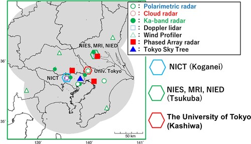
Fig. 1 Typical spatiotemporal scales of some examples of weather and climate phenomena. The numerical weather prediction model (NWP), general circulation model (GCM), and global cloud resolving model (GCRM) cover different but partially overlapping scales.

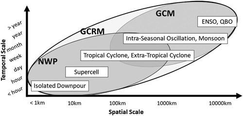
Fig. 2 Cloud images calculated by the GCRMs in the DYAMOND project and from the geostationary satellite Himawari-8 (After Fig. 2 in Stevens et al., 2019). From left to right: IFS with a horizontal resolution of 4, 9 km, and NICAM (top row); ARPEGE-NH, Himawari-8, and ICON (second row); FV3, GEOS5, and UM (third row); and SAM and MPAS (bottom row).

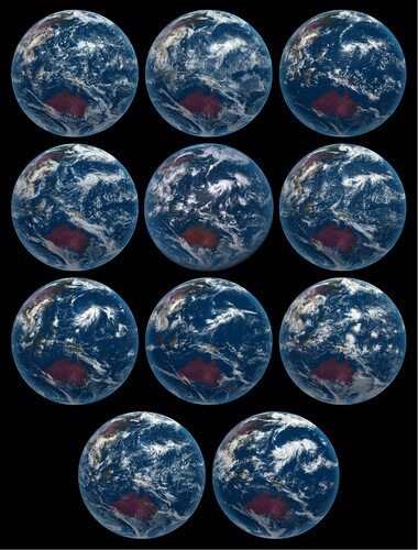
Table 2. List of GCRMs. Short names and references to the model-frameworks and recent settings are summarized. Cloud microphysics schemes in the DYAMOND GCRMs refer to the schemes used for the DYAMOND project. The subscripts v, c, r, i, s, and g indicate vapor, cloud water, rain, cloud ice, snow, and graupel categories, respectively.

Model name	References	Cloud microphysics schemes
ARPEGE-NH	Bubnová et al. (1995) Voldoire et al. (2017)	SMB with five categories (v, c, r, i, and s) Roehrig et al. (2020)
FV3	Lin and Rood (1997), Lin (2004), Zhou et al. (2019)	SMB with six categories (v, c, r, i, s, and g) Lin et al. (1983), Zhou et al. (2019)
GEOS5	Putman and Lin (2007), Putman and Suarez (2011), Arnold et al. (2020)	SMB with six categories (v, c, r, i, s, and g) Lin et al. (1983), Zhou et al. (2019)
GRIST	Zhang et al. (2019b; 2020b)	SMB with six categories (v, c, r, i, s, and g) Lin et al. (1983), Zhou et al. (2020)
ICON	Zängl et al. (2015), Hohenegger et al. (2020)	SMB with six categories (v, c, r, i, s, and g) Lin et al. (1983), Baldauf et al. (2011)
IFS	Malardel et al. (2016), Dueben et al. (2020), Wedi et al. (2020)	SMB with five categories (v, c, r, i, and s) Forbes et al. (2011)
MSSG	Takahashi et al. (2008), Sasaki et al. (2016), Onishi et al. (2019)	Bin microphysics for liquid particles and SMB for ice categories (v, liquid, i, s, g) Onishi and Takahashi (2012)
MPAS	Skamarock et al. (2012)	Hybrid of SMB and DMB with six categories [v, c, r, i, s, and g (the number concentrations of rain and cloud ice are predicted with prescribed aerosols)] Thompson et al. (2008) modified for WRF 3.8.1. (WRF User's Guide, n.d.)
NICAM	Satoh et al. (2014), Kodama et al. (2021)	SMB with six categories (v, c, r, i, s, and g) Lin et al. (1983), Tomita (2008b), Roh and Satoh (2014)
SAM	Khairoutdinov and Randall (2003), Satoh et al. (2019)	SMB with six categories [v, c, r, i, s, and g (ice categories are diagnosed)] Khairoutdinov and Randall (2003)
UM	Wood et al. (2014), Walters et al. (2019)	SMB with four categories [v, c, r, and i (cloud number concentration is diagnosed with climatological distribution of aerosols)] Wilson and Ballard (1999), Boutle et al. (2014), Walters et al. (2019)

Fig. 3 Cloud images calculated by the NICAM with horizontal resolutions of 14, 3.5 and 0.87 km (after Kajikawa et al., 2016). Zoom images of a tropical cyclone are shown in the right column.

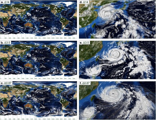
Fig. 4 A schematic image of the comparison between models and satellites using satellite simulators. From Masunaga et al. (2010), © American Meteorological Society. Used with permission.

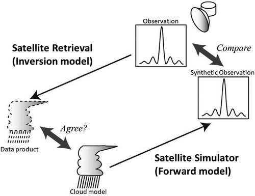
Fig. 5 Sample images of (a) the default NICAM with the global quasi-uniform icosahedral grid system, (b) stretched NICAM, and (c) diamond NICAM (after Uchida et al., 2017, © American Meteorological Society. Used with permission.).

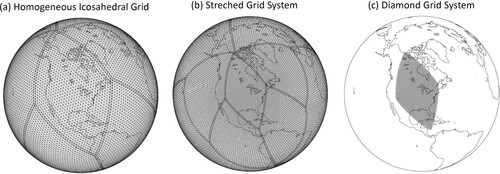
Fig. 6 Comparison of the vertical profiles of annual mean ice water content (IWC) [mg m-3] from (a) CloudSat satellite observations [2B-CWC-RO product (Austin et al., 2009; Austin & Stephens, 2001)], (b) NSW6 in NICAM.12, (c) NSW6 in NICAM.16, and NDW6 in NICAM.16. The solid lines represent 273-K isotherms. The global simulation data with horizontal resolution of 14 km and 38 vertical layers were provided by courtesy of C. Kodama and A. T. Noda.

Fig. 7 Comparison of outgoing longwave radiation at the top of the atmosphere (OLR) from CERES satellite observations (solid lines with points) and NICAM simulations with various versions of NDW6 (solid lines) (after Satoh et al., 2018).

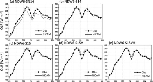
Fig. 8 The vertical profiles of (a) downward shortwave radiation and (b) upward shortwave radiation (after Seiki et al., 2014). Thick lines indicate observations by radiometer sonde, thin solid lines indicate NICAM simulations using NDW6 with spherical SSPs, and thin dashed lines indicate NICAM simulations using NDW6 with nonspherical SSPs. The dashed rectangles indicate the location of a cirrus layer.

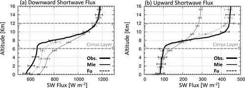
Fig. 9 Comparison of (a) OLR and (b) outgoing shortwave radiation at the top of the atmosphere (OSR) from CERES satellite observations (solid lines) and NICAM.16 simulations with various settings of cloud and radiation coupling. NSW6 uses full coupling between cloud and radiation (dashed lines), NSW6-Mie assumes variable effective radii but spherical SSPs (long dashed short dashed lines), and NSW6-Mie-ReFIX assumes constant effective radii and spherical SSPs (dotted lines). The global simulation data were provided by courtesy of C. Kodama.

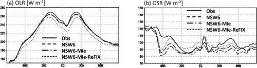
Fig. 10 Cloud microphysical processes and cloud interaction among water classes (after Satoh et al., 2018). Solid lines indicate the processes that change the number and mass concentration of hydrometeors, while dashed lines indicate the processes that change only the mass concentration of hydrometeors. Hom/het indicates homogeneous/heterogeneous, respectively.

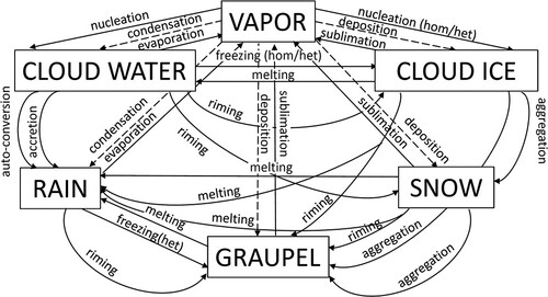
Table 3. Dependences of cloud-related processes on bulk cloud microphysical parameters.

Processes	Dependences	References	Assumptions
Auto-conversion (c → r)	$\rho \frac{\mathrm{\partial }{q}_c}{\mathrm{\partial }t}\propto (\rho q_c{)}^2{\overline{D_c}}^6$	Seifert and Beheng (2001)	Long’s kernel (Long, 1974) is used for the collection efficiency.
Auto-conversion (i → s)	$\rho \frac{\mathrm{\partial }{q}_i}{\mathrm{\partial }t}\propto \rho q_i{n}_i{\overline{D_i}}^4$	Seiki et al. (2015a)	Cloud ice is assumed to be spherical and sufficiently small to satisfy Stoke’s law. $v_{t,i}\propto D^2$
Riming (c → j) (j = i, s, g)	$\rho \frac{\mathrm{\partial }{q}_j}{\mathrm{\partial }t}\propto \rho q_c{n}_j{\overline{D_j}}^{2+d}$	Seiki and Roh (2020)	Power law is assumed between vt and D as follows: $v_t\propto D^d$with d typically ranging from 0.1–0.5 (e.g. Locatelli & Hobbs, 1974).
Condensation Evaporation Vapor Deposition Sublimation Melting	$\rho \frac{\mathrm{\partial }{q}_j}{\mathrm{\partial }t}\propto n_j\overline{D_j}$	Igel et al. (2015) Seiki and Roh (2020)	Spherical shape is assumed for ice particles.
Immersion freezing	$\rho \frac{\mathrm{\partial }{q}_r}{\mathrm{\partial }t}\propto \rho q_r{\overline{D_r}}^3$	Bigg (1953)	The equation is derived from experiment.
Cloud optical thickness τc	${\tau }_c\propto n_c{\overline{D_c}}^2$	Liou (2002)	Extinction efficiency is assumed to be approximately constant (2) for most particles.
Visible cloud albedo Rc	$R_c=\frac{\sqrt{3}\left(1-g\right){\tau }_c}{2+\sqrt{3}\left(1-g\right){\tau }_c}$	Liou (2002) Fu (2007)	Two-stream approximation is used with the asymmetry factor g typically ranging from 0.75–0.9 (e.g. Fu, 2007)
Infrared emissivity of cirrus εIR	${ϵ}_{IR}=1-\mathrm{e}\mathrm{x}\mathrm{p}\left(-0.79{\tau }_c\right)$	Fu and Liou (1993)	The function is derived by fitting to results from a numerical model with experimental data.

Table 4. Optical sensors and corresponding sensitive physical parameters.

Optical sensors	Satellites/instruments	Physical parameters
Visible/near-infrared imager (0.3–4 μm)	Geostationary meteorological satellites (e.g. GOES, Himawari, Meteosat), NOAA/AVHRR, Aqua, Terra/MODIS, GCOM-C/SGLI, TRMM-VIRS	Cloud optical thickness, Cloud-top effective radius
Infrared imager (8–12 μm)		Cloud-top temperature, Ice cloud optical thickness Ice cloud-top effective radius
Microwave imager (10–20 GHz)	Aqua/AMSR-E, GCOM-W/AMSR2, TRMM/TMI, GPM/GMI	Liquid water path, Precipitation flux,
Microwave imager (80–90 GHz)		Ice water path
Lidar (532, 1064 nm)	CALIPSO/CALIOP	Thermodynamic phase, Ice shape, Optical thickness
Cloud radar (94 GHz)	CloudSat/CPR	Ice water content, Liquid water content
Precipitation radar (13.6, 35.5 GHz)	TRMM/PR, GPM/DPR	Precipitation flux, Hydrometeor class

Fig. 11 Breakdown of OLR change under global warming simulated by the NICAM (after Noda et al., 2016). An OLR change ΔF is attributed to a change in emissivity Δε, a change in cloud-top temperature ΔT_CT, and a change in clear sky radiation ΔF^CLR. The breakdown was calculated by cloud size. Sum shows the summation of the contributions and the difference between ΔF and Sum indicates the error of the analysis.

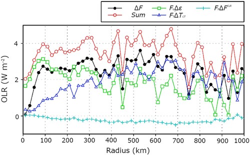
Fig. 12 The cloud-top and rain-top diagram using Ku-band radar echo and infrared brightness temperature from (a) satellite observations, (c) NSW6 in NICAM.12, and (e) NSW6 in NICAM.16. CFAD using Ku-band radar echo from (b) satellite observations, (d) NSW6 in NICAM.12, and (f) NSW6 in NICAM.16. Here, simulated results were processed by a Joint-Simulator. From Roh et al. (2017), © American Meteorological Society. Used with permission.

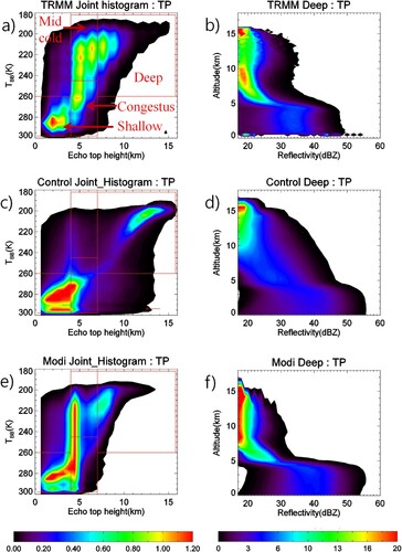
Fig. 13 Joint probability density function of the depolarization ratio δ and the ratio of attenuated backscattering coefficients for successive layers x from (a) satellite observations, (b) NSW6 in NICAM.16, and (c) NDW6. Low-level clouds behind a frontal cloud system were sampled over the Southern Ocean. Signals of supercooled liquid water are highlighted by circles. From Roh et al. (2020), © American Meteorological Society. Used with permission.

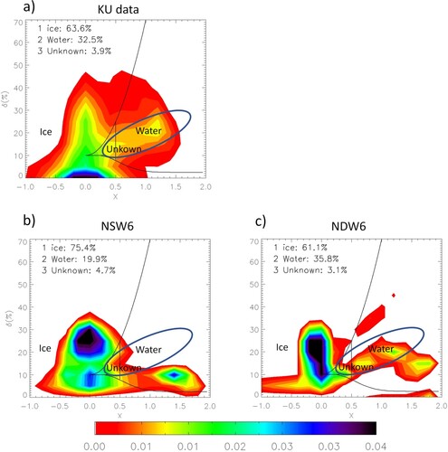
Fig. 14 Observation geometry of the EarthCARE satellite (from https://www.eorc.jaxa.jp/EARTHCARE/museum/poster_gallary.html, ©JAXA).

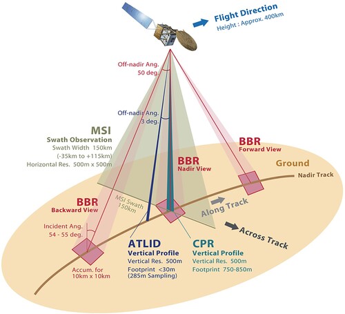
Fig. 15 Overview of the ground observations used in the ULTIMATE project around the Tokyo metropolitan area.

Stevens, B., Satoh, M., Auger, L., Biercamp, J., Bretherton, C. S., Chen, X., Düben, P., Judt, F., Khairoutdinov, M., Klocke, D., Kodama, C., Kornblueh, L., Lin, S.-J., Neumann, P., Putman, W. M., Röber, N., Shibuya, R., Vanniere, B., Vidale, P. L., … Zhou, L. (2019). DYAMOND: The DYnamics of the Atmospheric general circulation Modeled On Non-hydrostatic domains. Progress in Earth and Planetary Science, 6(1), 1–17. https://doi.org/10.1186/s40645-019-0304-z

 Web of Science ®Google Scholar

Bubnová, R., Hello, G., Bénard, P., & Geleyn, J.-F. (1995). Integration of the fully elastic equations cast in the hydrostatic pressure terrain-following coordinate in the framework of the ARPEGE/aladin NWP system. Monthly Weather Review, 123(2), 515–535. https://doi.org/10.1175/1520-0493(1995)123<0515:IOTFEE>2.0.CO;2

 Web of Science ®Google Scholar

Voldoire, A., Decharme, B., Pianezze, J., Lebeaupin Brossier, C., Sevault, F., Seyfried, L., Garnier, V., Bielli, S., Valcke, S., Alias, A., Accensi, M., Ardhuin, F., Bouin, M.-N., Ducrocq, V., Faroux, S., Giordani, H., Léger, F., Marsaleix, P., Rainaud, R., … Riette, S. (2017). SURFEX v8.0 interface with OASIS3-MCT to couple atmosphere with hydrology, ocean, waves and sea-ice models, from coastal to global scales. Geoscientific Model Development, 10(11), 4207–4227. https://doi.org/10.5194/gmd-10-4207-2017

 Web of Science ®Google Scholar

Roehrig, R., Beau, I., Saint-Martin, D., Alias, A., Decharme, B., Guérémy, J.-F., Voldoire, A., Abdel-Lathif, A. Y., Bazile, E., Belamari, S., Blein, S., Bouniol, D., Bouteloup, Y., Cattiaux, J., Chauvin, F., Chevallier, M., Colin, J., Douville, H., Marquet, P., … Sénési, S. (2020). The CNRM Global Atmosphere Model ARPEGE-Climat 6.3: Description and evaluation. Journal of Advances in Modeling Earth Systems, 12(7), 1–53. https://doi.org/10.1029/2020MS002075

 Web of Science ®Google Scholar

Lin, S.-J., & Rood, R. B. (1997). An explicit flux-form semi-lagrangian shallow-water model on the sphere. Quarterly Journal of the Royal Meteorological Society, 123(544), 2477–2498. https://doi.org/10.1002/qj.49712354416

 Web of Science ®Google Scholar

Lin, S.-J. (2004). A “Vertically lagrangian” Finite-Volume dynamical core for Global models. Monthly Weather Review, 132(10), 2293–2307. https://doi.org/10.1175/1520-0493(2004)132<2293:AVLFDC>2.0.CO;2

 Web of Science ®Google Scholar

Zhou, L., Lin, S.-J., Chen, J.-H., Harris, L. M., Chen, X., & Rees, S. L. (2019). Toward Convective-Scale prediction within the Next Generation Global prediction system. Bulletin of the American Meteorological Society, 100(7), 1225–1243. https://doi.org/10.1175/BAMS-D-17-0246.1

 Web of Science ®Google Scholar

Lin, Y.-L., Farley, R. D., & Orville, H. D. (1983). Bulk Parameterization of the snow field in a cloud model. Journal of Applied Meteorology and Climatology, 22(6), 1065–1092. https://doi.org/10.1175/1520-0450(1983)022<1065:BPOTSF>2.0.CO;2

 Google Scholar

Putman, W. M., & Lin, S.-J. (2007). Finite-volume transport on various cubed-sphere grids. Journal of Computational Physics, 227(1), 55–78. https://doi.org/10.1016/j.jcp.2007.07.022

 Web of Science ®Google Scholar

Putman, W. M., & Suarez, M. (2011). Cloud-system resolving simulations with the NASA Goddard Earth Observing system global atmospheric model (GEOS-5). Geophysical Research Letters, 38(16), 1–5. https://doi.org/10.1029/2011GL048438

 Google Scholar

Arnold, N. P., Putman, W. M., & Freitas, S. R. (2020). Impact of resolution and parameterized convection on the diurnal cycle of precipitation in a global nonhydrostatic model. Journal of the Meteorological Society of Japan. Ser. II, 98(6), 1279–1304. https://doi.org/10.2151/jmsj.2020-066

 Web of Science ®Google Scholar

Zhang, Y., Li, J., Yu, R., Zhang, S., Liu, Z., Huang, J., & Zhou, Y. (2019b). A layer-averaged Nonhydrostatic dynamical framework on an Unstructured Mesh for Global and regional Atmospheric Modeling: Model description, baseline evaluation, and sensitivity exploration. Journal of Advances in Modeling Earth Systems, 11(6), 1685–1714. https://doi.org/10.1029/2018MS001539

 Web of Science ®Google Scholar

Zhang, Y., Li, J., Yu, R., Liu, Z., Zhou, Y., Li, X., & Huang, X. (2020b). A Multiscale dynamical Model in a Dry-mass Coordinate for Weather and Climate Modeling: Moist Dynamics and Its coupling to physics. Monthly Weather Review, 148(7), 2671–2699. https://doi.org/10.1175/MWR-D-19-0305.1

 Web of Science ®Google Scholar

Zängl, G., Reinert, D., Rípodas, P., & Baldauf, M. (2015). The ICON (ICOsahedral Non-hydrostatic) modelling framework of DWD and MPI-M: Description of the non-hydrostatic dynamical core. Quarterly Journal of the Royal Meteorological Society, 141(687), 563–579. https://doi.org/10.1002/qj.2378

 Web of Science ®Google Scholar

Hohenegger, C., Kornblueh, L., Klocke, D., Becker, T., Cioni, G., Engels, J. F., Schulzweida, U., & Stevens, B. (2020). Climate Statistics in Global simulations of the atmosphere, from 80 to 2.5 km grid spacing. Journal of the Meteorological Society of Japan. Ser. II, 98(1), 73–91. https://doi.org/10.2151/jmsj.2020-005

 Web of Science ®Google Scholar

Baldauf, M., Seifert, A., Förstner, J., Majewski, D., Raschendorfer, M., & Reinhardt, T. (2011). Operational convective-scale numerical weather prediction with the COSMO model: description and sensitivities. Monthly Weather Review, 139(12), 3887–3905. https://doi.org/10.1175/MWR-D-10-05013.1

 Web of Science ®Google Scholar

Malardel, S., Wedi, N., Deconinck, W., Diamantakis, M., Kuehnlein, C., Mozdzynski, G., Hamrud, M., & Smolarkiewicz, P. (2016). A new grid for the IFS. ECMWF. https://doi.org/10.21957/zwdu9u5i

 Google Scholar

Dueben, P. D., Wedi, N., Saarinen, S., & Zeman, C. (2020). Global simulations of the Atmosphere at 1.45 km grid-spacing with the integrated forecasting system. Journal of the Meteorological Society of Japan. Ser. II, 98(3), 551–572. https://doi.org/10.2151/jmsj.2020-016

 Web of Science ®Google Scholar

Wedi, N. P., Polichtchouk, I., Dueben, P., Anantharaj, V. G., Bauer, P., Boussetta, S., Browne, P., Deconinck, W., Gaudin, W., Hadade, I., Hatfield, S., Iffrig, O., Lopez, P., Maciel, P., Mueller, A., Saarinen, S., Sandu, I., Quintino, T., & Vitart, F. (2020). A baseline for Global Weather and Climate simulations at 1 km resolution. Journal of Advances in Modeling Earth Systems, 12(11), 1–17. https://doi.org/10.1029/2020MS002192

 Web of Science ®Google Scholar

Forbes, R., Tompkins, A. M., & Untch, A. (2011). A new prognostic bulk microphysics scheme for the IFS. ECMWF. https://doi.org/10.21957/bf6vjvxk

 Google Scholar

Takahashi, K., Peng, X., Onishi, R., Ohdaira, M., Goto, K., Fuchigami, H., & Sugimura, T. (2008). Impact of coupled Nonhydrostatic atmosphere-ocean-land model with high resolution. In K. Hamilton, & W. Ohfuchi (Eds.), High Resolution Numerical Modelling of the Atmosphere and ocean (pp. 261–273). Springer. https://doi.org/10.1007/978-0-387-49791-4_15

 Google Scholar

Sasaki, W., Onishi, R., Fuchigami, H., Goto, K., Nishikawa, S., Ishikawa, Y., & Takahashi, K. (2016). MJO simulation in a cloud-system-resolving global ocean-atmosphere coupled model. Geophysical Research Letters, 43(17), 9352–9360. https://doi.org/10.1002/2016GL070550

 Web of Science ®Google Scholar

Onishi, R., Sugiyama, D., & Matsuda, K. (2019). Super-Resolution simulation for real-time prediction of urban micrometeorology. Sola, 15(0), 178–182. https://doi.org/10.2151/sola.2019-032

 Google Scholar

Onishi, R., & Takahashi, K. (2012). A warm-Bin–cold-bulk hybrid cloud microphysical model. Journal of the Atmospheric Sciences, 69(5), 1474–1497. https://doi.org/10.1175/JAS-D-11-0166.1

 Web of Science ®Google Scholar

Skamarock, W. C., Klemp, J. B., Duda, M. G., Fowler, L. D., Park, S.-H., & Ringler, T. D. (2012). A Multiscale Nonhydrostatic Atmospheric Model using centroidal voronoi tesselations and C-grid staggering. Monthly Weather Review, 140(9), 3090–3105. https://doi.org/10.1175/MWR-D-11-00215.1

 Web of Science ®Google Scholar

Thompson, G., Field, P. R., Rasmussen, R. M., & Hall, W. D. (2008). Explicit forecasts of Winter Precipitation using an improved bulk microphysics scheme. Part II: Implementation of a New snow parameterization. Monthly Weather Review, 136(12), 5095–5115. https://doi.org/10.1175/2008MWR2387.1

 Web of Science ®Google Scholar

WRF Users’ Guide. (n.d.). Retrieved May 19, 2021, from https://www2.mmm.ucar.edu/wrf/users/docs/user_guide_V3/user_guide_V3.8/contents.html

 Google Scholar

Satoh, M., Tomita, H., Yashiro, H., Miura, H., Kodama, C., Seiki, T., Noda, A. T., Yamada, Y., Goto, D., Sawada, M., Miyoshi, T., Niwa, Y., Hara, M., Ohno, T., Iga, S., Arakawa, T., Inoue, T., & Kubokawa, H. (2014). The Non-hydrostatic icosahedral Atmospheric model: Description and development. Progress in Earth and Planetary Science, 1(1), 1–32. https://doi.org/10.1186/s40645-014-0018-1

 Google Scholar

Kodama, C., Ohno, T., Seiki, T., Yashiro, H., Noda, A. T., Nakano, M., Yamada, Y., Roh, W., Satoh, M., Nitta, T., Goto, D., Miura, H., Nasuno, T., Miyakawa, T., Chen, Y.-W., & Sugi, M. (2021). The Nonhydrostatic ICosahedral Atmospheric Model for CMIP6 HighResMIP simulations (NICAM16-S): experimental design, model description, and impacts of model updates. Geoscientific Model Development, 14(2), 795–820. https://doi.org/10.5194/gmd-14-795-2021

 Web of Science ®Google Scholar

Tomita, H. (2008b). New microphysical schemes with five and Six categories by Diagnostic Generation of cloud Ice. Journal of the Meteorological Society of Japan. Ser. II, 86A, 121–142. https://doi.org/10.2151/jmsj.86A.121

 Web of Science ®Google Scholar

Roh, W., & Satoh, M. (2014). Evaluation of precipitating hydrometeor parameterizations in a single-moment Bulk Microphysics scheme for deep convective systems over the tropical central pacific. Journal of the Atmospheric Sciences, 71(7), 2654–2673. https://doi.org/10.1175/JAS-D-13-0252.1

 Web of Science ®Google Scholar

Khairoutdinov, M. F., & Randall, D. A. (2003). Cloud Resolving Modeling of the ARM Summer 1997 IOP: Model formulation, results, uncertainties, and sensitivities. Journal of the Atmospheric Sciences, 60(4), 607–625. https://doi.org/10.1175/1520-0469(2003)060<0607:CRMOTA>2.0.CO;2

 Web of Science ®Google Scholar

Satoh, M., Stevens, B., Judt, F., Khairoutdinov, M., Lin, S.-J., Putman, W. M., & Düben, P. (2019). Global Cloud-Resolving models. Current Climate Change Reports, 5(3), 172–184. https://doi.org/10.1007/s40641-019-00131-0

 Web of Science ®Google Scholar

Wood, N., Staniforth, A., White, A., Allen, T., Diamantakis, M., Gross, M., Melvin, T., Smith, C., Vosper, S., Zerroukat, M., & Thuburn, J. (2014). An inherently mass-conserving semi-implicit semi-Lagrangian discretization of the deep-atmosphere global non-hydrostatic equations. Quarterly Journal of the Royal Meteorological Society, 140(682), 1505–1520. https://doi.org/10.1002/qj.2235

 Web of Science ®Google Scholar

Walters, D., Baran, A. J., Boutle, I., Brooks, M., Earnshaw, P., Edwards, J., Furtado, K., Hill, P., Lock, A., Manners, J., Morcrette, C., Mulcahy, J., Sanchez, C., Smith, C., Stratton, R., Tennant, W., Tomassini, L., Van Weverberg, K., Vosper, S., … Zerroukat, M. (2019). The Met Office Unified Model Global Atmosphere 7.0/7.1 and JULES Global land 7.0 configurations. Geoscientific Model Development, 12(5), 1909–1963. https://doi.org/10.5194/gmd-12-1909-2019

 Web of Science ®Google Scholar

Wilson, D. R., & Ballard, S. P. (1999). A microphysically based precipitation scheme for the UK meteorological office unified model. Quarterly Journal of the Royal Meteorological Society, 125(557), 1607–1636. https://doi.org/10.1002/qj.49712555707

 Web of Science ®Google Scholar

Boutle, I. A., Eyre, J. E. J., & Lock, A. P. (2014). Seamless stratocumulus simulation across the turbulent gray zone. Monthly Weather Review, 142(4), 1655–1668. https://doi.org/10.1175/MWR-D-13-00229.1

 Web of Science ®Google Scholar

Kajikawa, Y., Miyamoto, Y., Yoshida, R., Yamaura, T., Yashiro, H., & Tomita, H. (2016). Resolution dependence of deep convections in a global simulation from over 10-kilometer to sub-kilometer grid spacing. Progress in Earth and Planetary Science, 3(1), 1–14. https://doi.org/10.1186/s40645-016-0094-5

 Google Scholar

Masunaga, H., Matsui, T., Tao, W., Hou, A. Y., Kummerow, C. D., Nakajima, T., Bauer, P., Olson, W. S., Sekiguchi, M., & Nakajima, T. Y. (2010). Satellite Data Simulator Unit: a multisensor, multispectral satellite simulator package. Bulletin of the American Meteorological Society, 91(12), 1625–1632. https://doi.org/10.1175/2010BAMS2809.1

 Web of Science ®Google Scholar

Uchida, J., Mori, M., Hara, M., Satoh, M., Goto, D., Kataoka, T., Suzuki, K., & Nakajima, T. (2017). Impact of lateral Boundary Errors on the simulation of clouds with a Nonhydrostatic regional Climate model. Monthly Weather Review, 145(12), 5059–5082. https://doi.org/10.1175/MWR-D-17-0158.1

 Web of Science ®Google Scholar

Austin, R. T., Heymsfield, A. J., & Stephens, G. L. (2009). Retrieval of ice cloud microphysical parameters using the CloudSat millimeter-wave radar and temperature. Journal of Geophysical Research: Atmospheres, 114(D8), 1–19. https://doi.org/10.1029/2008JD010049

 Google Scholar

Austin, R. T., & Stephens, G. L. (2001). Retrieval of stratus cloud microphysical parameters using millimeter-wave radar and visible optical depth in preparation for CloudSat: 1. Algorithm formulation. Journal of Geophysical Research: Atmospheres, 106(D22), 28233–28242. https://doi.org/10.1029/2000JD000293

 Web of Science ®Google Scholar

Satoh, M., Noda, A. T., Seiki, T., Chen, Y.-W., Kodama, C., Yamada, Y., Kuba, N., & Sato, Y. (2018). Toward reduction of the uncertainties in climate sensitivity due to cloud processes using a global non-hydrostatic atmospheric model. Progress in Earth and Planetary Science, 5(1), 1–29. https://doi.org/10.1186/s40645-018-0226-1

 Google Scholar

Seiki, T., Satoh, M., Tomita, H., & Nakajima, T. (2014). Simultaneous evaluation of ice cloud microphysics and nonsphericity of the cloud optical properties using hydrometeor video sonde and radiometer sonde in situ observations. Journal of Geophysical Research: Atmospheres, 119(11), 6681–6701. https://doi.org/10.1002/2013JD021086

 Web of Science ®Google Scholar

Seifert, A., & Beheng, K. D. (2001). A double-moment parameterization for simulating autoconversion, accretion and selfcollection. Atmospheric Research, 59–60, 265–281. https://doi.org/10.1016/S0169-8095(01)00126-0

 Web of Science ®Google Scholar

Long, A. B. (1974). Solutions to the droplet collection equation for polynomial kernels. Journal of the Atmospheric Sciences, 31(4), 1040–1052. https://doi.org/10.1175/1520-0469(1974)031<1040:STTDCE>2.0.CO;2

 Web of Science ®Google Scholar

Seiki, T., Kodama, C., Noda, A. T., & Satoh, M. (2015a). Improvement in Global cloud-system-resolving simulations by using a double-moment bulk cloud microphysics scheme. Journal of Climate, 28(6), 2405–2419. https://doi.org/10.1175/JCLI-D-14-00241.1

 Web of Science ®Google Scholar

Seiki, T., & Roh, W. (2020). Improvements in supercooled liquid water simulations of Low-level mixed-phase clouds over the Southern Ocean using a single-column model. Journal of the Atmospheric Sciences, 77(11), 3803–3819. https://doi.org/10.1175/JAS-D-19-0266.1

 Web of Science ®Google Scholar

Locatelli, J. D., & Hobbs, P. V. (1974). Fall speeds and masses of solid precipitation particles. Journal of Geophysical Research (1896-1977), 79(15), 2185–2197. https://doi.org/10.1029/JC079i015p02185

 Google Scholar

Igel, A. L., Igel, M. R., & Heever, S. C. v. d. (2015). Make It a double? Sobering results from simulations using single-moment microphysics schemes. Journal of the Atmospheric Sciences, 72(2), 910–925. https://doi.org/10.1175/JAS-D-14-0107.1

 Web of Science ®Google Scholar

Bigg, E. K. (1953). The formation of atmospheric ice crystals by the freezing of droplets. Quarterly Journal of the Royal Meteorological Society, 79(342), 510–519. https://doi.org/10.1002/qj.49707934207

 Web of Science ®Google Scholar

Liou, K. N. (2002). An introduction to Atmospheric radiation. Elsevier.

 Google Scholar

Fu, Q. (2007). A New Parameterization of an asymmetry factor of cirrus clouds for climate models. Journal of the Atmospheric Sciences, 64(11), 4140–4150. https://doi.org/10.1175/2007JAS2289.1

 Web of Science ®Google Scholar

Fu, Q., & Liou, K. N. (1993). Parameterization of the Radiative Properties of Cirrus clouds. Journal of the Atmospheric Sciences, 50(13), 2008–2025. https://doi.org/10.1175/1520-0469(1993)050<2008:POTRPO>2.0.CO;2

 Web of Science ®Google Scholar

Noda, A. T., Seiki, T., Satoh, M., & Yamada, Y. (2016). High cloud size dependency in the applicability of the fixed anvil temperature hypothesis using global nonhydrostatic simulations. Geophysical Research Letters, 43(5), 2307–2314. https://doi.org/10.1002/2016GL067742

 Web of Science ®Google Scholar

Roh, W., Satoh, M., & Nasuno, T. (2017). Improvement of a cloud microphysics scheme for a Global Nonhydrostatic Model Using TRMM and a satellite simulator. Journal of the Atmospheric Sciences, 74(1), 167–184. https://doi.org/10.1175/JAS-D-16-0027.1

 Web of Science ®Google Scholar

Roh, W., Satoh, M., Hashino, T., Okamoto, H., & Seiki, T. (2020). Evaluations of the thermodynamic Phases of clouds in a Cloud-System-Resolving Model Using CALIPSO and a satellite simulator over the Southern Ocean. Journal of the Atmospheric Sciences, 77(11), 3781–3801. https://doi.org/10.1175/JAS-D-19-0273.1

 Web of Science ®Google Scholar