The Pleistocene Glacial Cycles and Millennial-Scale Climate Variability

Figures & data

Fig. 1 The primary record of the past climate is the ${\delta }^{18}O$ of benthic foraminifera in the deep sea sediments. Top curve in the left panel shows the stacked record of the past 2 Myr (Lisiecki & Raymo, 2005). The record has a dominant cyclicity with a period of 41 kyr prior to the MPT around 1 My BP. After the MPT the glacial cycles became more irregular and lasting approximately 100 kyr. The difference between the two periods is manifested in the power spectra, which show a strong spectral peak at 41 kyr and very little power around 100 kyr prior to the MPT (top right, first panel), while a broad spectral peak occurs around 100 kyr after the MPT, but still with some power in the 41 kyr peak. The orbital parameters and the 65N ss insolation are shown below. For these the spectra before and after the MPT are essentially identical, as seen in the right panels. The vertical red lines indicates periods of 23 kyr (precession), 41 kyr (obliquity) and 100 kyr (eccentricity).

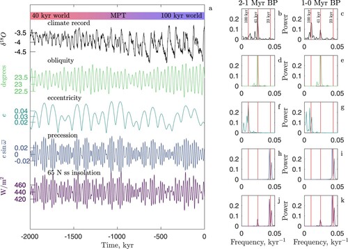
Fig. 2 The climate record (Lisiecki & Raymo, 2005) for the past 1 My is compared with a few of the proposed models. In each of the models a small intensity, $\sigma =0.02$ stochastic forcing is applied. In the Imbrie and Imbrie, 1980 model the timescales for glaciation and deglaciation are ${\tau }_1=50$ kyr and ${\tau }_2=2$ kyr (Eq. (1(1) $\mathrm{d}y/\mathrm{d}t=(x-y)/\tau .$(1) )). The Saltzman and Maasch, 1991 model (Eq. (3(3) $\begin{array}{rll}\mathrm{d}I/\mathrm{d}\tau & =-I-\mu -{\alpha }_1\theta -{\alpha }_{2}F\left(\tau \right)+{\eta }_I\left(t\right)& \\ \mathrm{d}\mu /\mathrm{d}\tau & =-{\text{β}}_1\theta +{\text{β}}_2\mu -{\text{β}}_3{\mu }^2-{\mu }^3+{\eta }_{\mu }\left(t\right)\\ \mathrm{d}\theta /\mathrm{d}\tau & =-{\gamma }_1(I+\theta )+{\eta }_{\theta }\left(t\right),\end{array}$(3) )) is shown with parameters $({\alpha }_1,{\text{β}}_1,{\text{β}}_2,{\text{β}}_3,{\gamma }_1)=(1.0,2.5,1.3,0.6,0.2)$ and in the two cases ${\alpha }_2=0$ i.e. no astronomical forcing and ${\alpha }_2=0.5$ with the astronomical forcing $F\left(\tau \right)$ being the 65 N ss insolation normalized to zero mean and unit variance. The dimensionless time is $\tau =t/10$ kyr. The Huybers and Wunch, 2005 model has a linear drift, which in the case of no noise would produce a glaciation of 90 kyr and a deglaciation of 10 kyr.

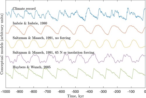
Fig. 3 The MPT is assumed to be caused by a slow, tectonic timescale change in conditions, represented by a “control parameter”, which changes across the MPT (top blue curve). There is no change in the astronomical forcing, here represented by a harmonic 41 kyr oscillation, representing the obliquity. The noisy climate record (Lisiecki & Raymo, 2005) change from 40 kyr to 100 kyr cycles at the MPT. The models are reacting to the changing control parameter and the forcing in dynamically different ways: In the Saltzman & Maasch model (Eq. (3(3) $\begin{array}{rll}\mathrm{d}I/\mathrm{d}\tau & =-I-\mu -{\alpha }_1\theta -{\alpha }_{2}F\left(\tau \right)+{\eta }_I\left(t\right)& \\ \mathrm{d}\mu /\mathrm{d}\tau & =-{\text{β}}_1\theta +{\text{β}}_2\mu -{\text{β}}_3{\mu }^2-{\mu }^3+{\eta }_{\mu }\left(t\right)\\ \mathrm{d}\theta /\mathrm{d}\tau & =-{\gamma }_1(I+\theta )+{\eta }_{\theta }\left(t\right),\end{array}$(3) )) the parameter ${\text{β}}_1$ changes linearly with the control parameter and the model undergoes a Hopf-bifurcation from a fixed point before the MPT to a limit cycle after the MPT. The astronomical forcing results just in a linear response (solutions with and without forcing are shown). In the Van der Pol oscillator the slowly changing parameter controls the period of the oscillator, which is longer than 41 kyr. The oscillator locks to the forcing which, when the internal frequency becomes much longer than the period of the forcing results in a 2:1 and 3:1 frequency locking. In the Paillard model the control parameter determines the threshold ice volume after which the climate will jump into the deep glacial state. In the Ashwin & Ditlevsen model, the system undergoes a transcritical transition at the MPT.

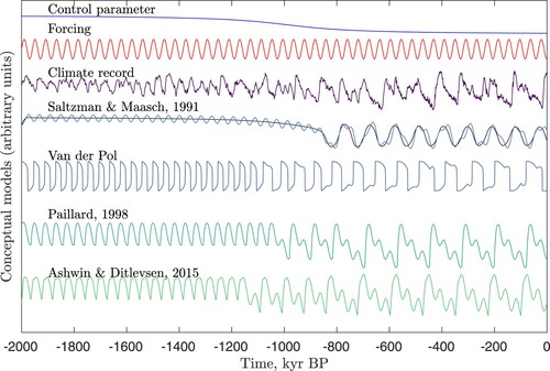
Fig. 4 The power spectrum of the climate record where the continuous part of the spectrum is emphasised. The smooth curve is the power spectrum for the red noise or Ornstein-Uhlenbeck process with a correlation time of 100 kyr.

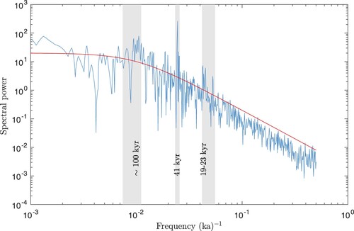
Fig. 5 Panel a. shows the NGRIP ${\delta }^{18}O$ climate record (North GRIP Members, 2004) at 20 yr resolution covering the past 120 kyr (top curve). The middle curve is the 150 years running mean (low pass), while the green curve is the high pass residual. The DO events are retained in the low pass signal, while the high pass signal contains decadal scale climate fluctuations, which are larger in the cold stadial climate than in the warm interstadial climate. A standard deviation for the two states are indicated by red lines in panel b. with is a blowup of the period indicated by the vertical grey bar in panel a. Panel c. is the power spectrum of the record, consistent with the power spectrum for the ocean sediment record in Fig. 4. For time scales around 150 yr the red noise spectrum, indicated by the red line, crosses over to a white noise spectrum, indicated by the blue line.

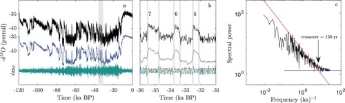
Fig. 6 The waiting time distribution in the period 60-20 kyr BP. Red circles are durations of stadial periods, corresponding to the waiting time before an abrupt jump into the interstadial state. The red line corresponds to an exponential distribution $P(t>\tau )=\exp -\tau /\overline{\tau }$, with mean waiting time $\overline{\tau }=1320$ yr. Black circles and lines are the same for the interstadials, with $\overline{\tau }=770$ yr.

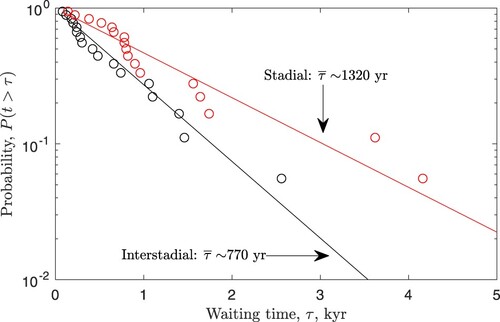
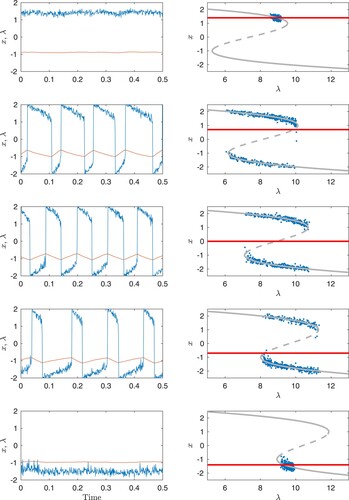
Fig. 7 Five realizations of the noisy FitzHugh-Nagumo model with different parameter values for $c_0$ (see text) and null-clines for $\mathrm{d}\lambda /\mathrm{d}t=0\Rightarrow x=c_0$. From bottom and up, $c_0$ is increasing from a situation where the cold climate state is stable, through an oscillator DO phase, to a situation where the warm climate state is stable. The grey curves where $\mathrm{d}x/\mathrm{d}t=0$ are the slow manifold. The blue curves in the left panels are $x\left(t\right)$, while the red curves are the slowly varying $\lambda \left(t\right)$. The blue dots in the right panels are scatter plots of $\left(x\right(t),\lambda (t\left)\right)$.

Lisiecki, L. E., & Raymo, M. E. (2005). A Pliocene-Pleistocene stack of 57 globally distributed benthic d18O records. Paleoceanography, 20(1), PA1003. https://doi.org/10.1029/2004PA001071.

 Google Scholar

North GRIP Members (2004). High resolution climate record of the Northern hemisphere reaching into the last glacial interglacial period. Nature, 431, 147–151. https://doi.org/10.1038/nature02805.

 PubMed Web of Science ®Google Scholar