Figures & data
Fig. 1 Types of remote sensing sensors and their wavelengths. (Adapted from , https://earth.esa.int/documents/10174/642943/6-LTC2013-SAR-Moreira.pdf).
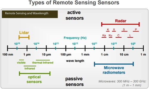
Fig. 2 Space-based component of the global observing system (source, WMO Space Program).
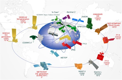
Fig. 3 The Geostationary Operational Environmental Satellite (GOES) R-Series satellite and instruments. Graphic courtesy of Lockheed Martin and the GOES-R Program.
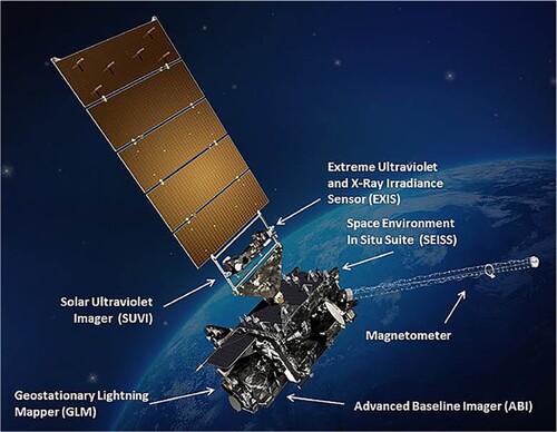
Fig. 4 The Joint Polar Satellite System (JPSS) satellite and instruments. Graphic courtesy of Joseph Smith and the JPSS Program.
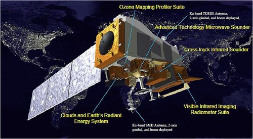
Table 1. Satellite backbone with specified orbital configuration and measurement approaches (Subcomponent 1), Source WMO WIGOS.
Table 2. Backbone satellite system with open orbit configuration and flexibility to optimize the implementation (Subcomponent 2, Source WMO WIGOS).
Table 3. The characteristics and uses of weather radars.
Fig. 5 NEXRAD/WSR88-D coverage at (a) 3 and (b) 1 km AGL at the centre of the beam at 0.5 deg elevation angle. Note how the coverage gets lower as the height above the ground decreases. While coverage is very good at midlevels over much of the U. S. east of the Rocky Mountains, it is much sparser in the boundary layer. (from McLaughlin et al., Citation2009).
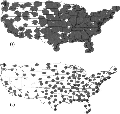
Fig. 6 Derived Motion Wind Vectors (DMW) from the GOES East (GOES-16) Advanced Baseline Imager overlaid on a GeoColor false colour RGB image (Miller et al., Citation2020) at 13 UTC on 21 October, 2020. At this time Category 1 Hurricane Epsilon in the north-central Atlantic (28.9°N, 58.8°W) has a well-defined cyclonic circulation, minimum pressure of 976 hPA, and maximum sustained winds of 74 kts (85mph). Source: NOAA, NESDIS GOES Imager Viewer.
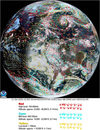
Fig. 7 Surface station plotting model (https://en.wikipedia.org/wiki/Station_model#/media/File:Station_model.gif).
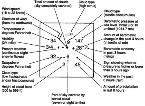
Fig. 8 Typical Automated Surface Observing System (ASOS). Courtesy of Kenneth Boutin, National Weather Service.
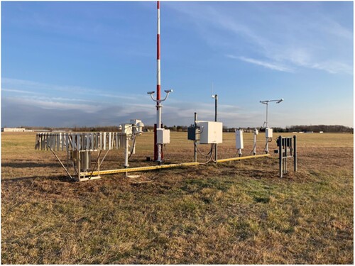
Fig. 9 RaXPol, a rapid-scan, X-band, polarimetric mobile Doppler radar scanning a tornado in Kansas in 2016. Courtesy of H. Bluestein.
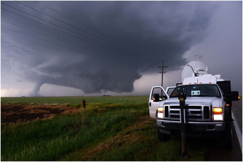
Fig. 10 CopterSonde UAS for atmospheric measurements made by the Center for Automated Sensing Systems at the University of Oklahoma. Photo courtesy of Tony Segalés.
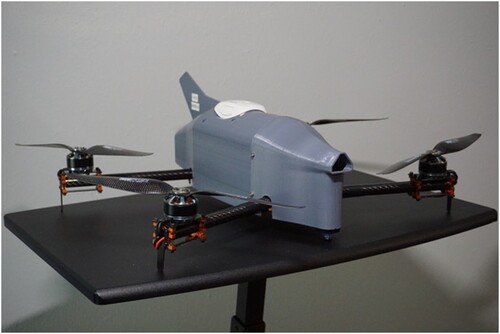
Fig. 11 NASA ER-2 instrumentation complement used in the GOES-16 post-launch test field campaign to validate the performance of the GOES-16 ABI and GLM (Padula et al., Citation2016). The VIRIS-NG is the Next-Generation Airborne Visible/Infrared Imaging Spectrometer, LIP is the Lightning Instrument Package (electric field-mills), EXRAD is the ER-2 x-band Doppler radar, CPL is the Cloud Physics Lidar, GCAS is the GeoCAPE Airborne Simulator, S-HIS is the High-resolution Interferometer Sounder, CRS is the 94 GHz (W-band) Cloud Radar System, and FEGS is the Fly’s Eye GLM Simulator. Refer to (https://airbornescience.nasa.gov/) for additional instrument details.
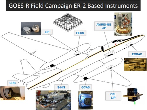
Table 4. NASA ER2 instrument complement used in the GOES-16 post-launch test campaign. The instrument specs include type of measurement, spectral range, spectral resolution, ground sample distance (GSD), field of view (FOV), and swath width.
Fig. 12 Forecast Sensitivity to Observations Impact (FSOI) ranking comparison (courtesy of Will McCarty, NASA Goddard Modeling and Data Assimilation Office (GMAO)).
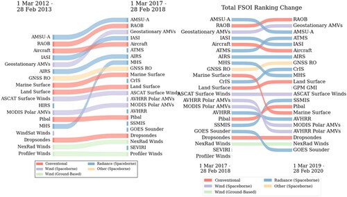
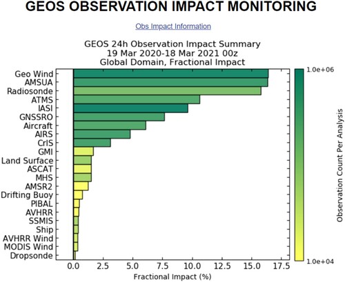
Fig. 13 Observation impacts computed using the adjoint of the Goddard Earth Observing System, Version 5 (GEOS-5) atmospheric data assimilation system at NASA GSFC. The average values for each observing system are shown over the full year 19 March 2020–18 March 2021. The values are averaged over the number of cases in the interval, and the colour shading denotes the average number of observations for a given observing system. Observation impacts in GEOS-5 are computed once each day for the 24-h forecast initialized at 00Z. The results shown are from the GEOS-5 interactive web page (https://gmao.gsfc.nasa.gov/forecasts/systems/fp/obs_impact/).