Figures & data
Fig. 1 Photos of cloud systems. (A) A mesoscale convective system over tropical continent. (B) A thunderstorm over tropical ocean. (C) Fair weather cumulus clouds over land. (D) Stratocumulus clouds over ocean. [Courtesy of NASA].
![Fig. 1 Photos of cloud systems. (A) A mesoscale convective system over tropical continent. (B) A thunderstorm over tropical ocean. (C) Fair weather cumulus clouds over land. (D) Stratocumulus clouds over ocean. [Courtesy of NASA].](/cms/asset/92ebf0da-d4ce-4e42-8138-5fc45c3e585e/tato_a_2082915_f0001_oc.jpg)
Fig. 2 Biases of climatological mean precipitation with respect to GPCP/TRMM observations for (A) Ensemble mean of 23 CMIP5 global climate models (Huang et al., Citation2018). (B) An AGCM with super-parameterization of convection (Randall et al., Citation2016). (C) A global cloud resolving model (Kodama et al., Citation2015); and (D) ERA5 reanalysis (Hersbach et al., Citation2020).
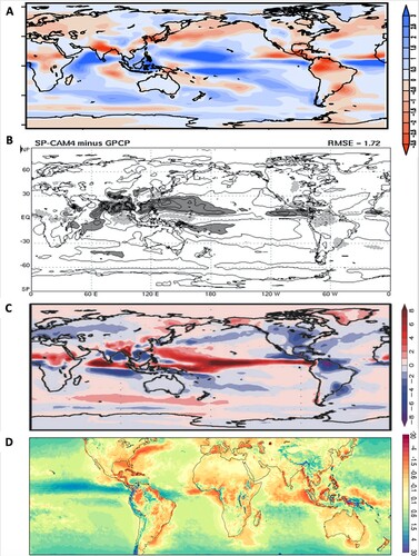
Fig. 3 (A) MJO precipitation variance in CMIP3 models (left, from Lin et al., Citation2006) and CMIP5 models (right, from Hung et al., Citation2013). (B) Phase and amplitude of diurnal cycle of precipitation over land (left) and ocean (right) for CMIP5 AMIP models and TRMM observations (adapted from Covey et al., Citation2016).
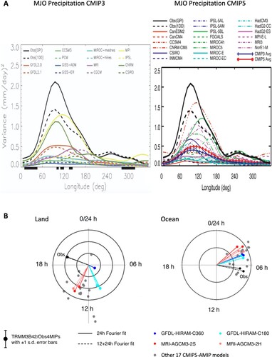
Table 1 Convection schemes used in global and regional models grouped by closure assumptions.
Fig. 4 (A) Average vertical velocity in the strongest 10% convective updrafts and downdrafts in oceanic convection comparing with Florida Thunderstorm Project data (from Black et al., Citation1996). (B) Average vertical velocity in the strongest 10% convective updrafts in Amazon and Southern Great Plain (SGP) (from Wang et al. 2020). (C) Same as A but for convective core width (from Lucas et al., Citation1994). (D) Same as B but for convective core width. (E) Global estimated entrainment rate binned by cloud top heights (from Stanfield et al., Citation2019). (F) Vertical profile of entrainment rate for TWP-Ice in Australia (from Zhang et al., Citation2016).
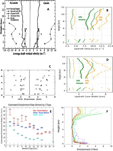
Fig. 5 Lag-regression of divergence profile with respect to surface precipitation for seven field experiments. Lag 0 is the time of maximum precipitation, and lag −10 (+10) hours means 10 h before (after) maximum precipitation. The locations of the field experiments are shown in the top map (from Mapes & Lin, Citation2005).
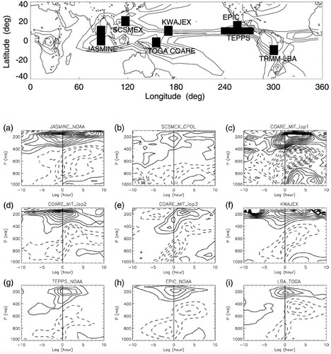
Fig. 6 (A) Circulation within an ordinary thunderstorm in (left) developing, (middle) mature, and (right) dissipating stages (adapted from Byers & Braham, Citation1948). (B) Visual model of the mature phase of a classic supercell thunderstorm (adapted from Bluestein & Parks, Citation1983). (C) Vertical cross-section of an MCC (adapted from Fortune et al., Citation1992). (D) Schematic cross-section of a squall line moving from right to left, and the post-convection sounding. Circled numbers are typical values of θw in °C (adapted from Zipser, Citation1977).
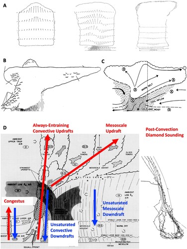
Fig. 7 (A) The GPCP climatological mean precipitation (contour interval 1.5 mm/day). The coloured boxes are regions used in b and c. (B) Normalized vertical distribution of TRMM precipitation radar 20 dBZ echo top for convective precipitation from 16 years of data (1998–2013). (C) Normalized Q1 profiles for NAME, TOGA COARE, DYNAMO and GATE.
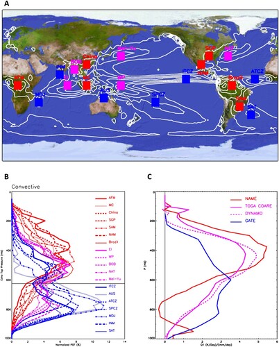
Fig. 8 (A) Normalized vertical distribution of TRMM precipitation radar 20 dBZ echo top for stratiform precipitation for regions shown in A. (B) Partitioning of GATE Q1 profile into convective, stratiform and radiative components (from Johnson, Citation1984). (C) TRMM PR convective and stratiform precipitation fractions for NH summer (from Yang & Smith, Citation2008). (D) CMIP5 model convective precipitation fraction for high-resolution and low-resolution ensemble means for NH summer (from Huang et al., Citation2018).
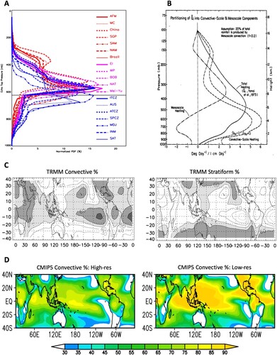
Fig. 9 (A) Global climatology of mesoscale cellular convection depicting the most favoured regions of open and closed mesoscale cellular convection over the oceans (from Agee, Citation1987). (B) Left: The observed Q1, Q2, QR, and Q1 − QR for the undisturbed BOMEX period 22–26 June 1969 (from Nitta & Esbensen, Citation1974). Right: Schematic of trade wind cumulus layer showing effects of condensation c and evaporation e on the heat and moisture budgets (from Johnson & Lin, Citation1997). (C) Left: Longwave heating rate of a stratocumulus-topped boundary layer (from Larson et al., Citation2007). Right: Schematic depiction of the large-scale forcing and physical processes for a stratocumulus-topped boundary layer. LTS is lower troposphere stability and EIS is estimated inversion strength (adapted from Lin et al., Citation2014).
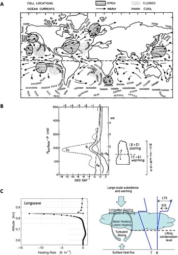
Fig. 10 Zonal momentum budget of the Walker Circulation, as shown by climatological annual mean (a) pressure gradient force, (b) Coriolis force, (c) advective tendency, and (d) convective eddy momentum flux convergence along the equator (5N-5S) derived from 15 years (1979–1993) of NCEP reanalysis data. Unit is m/s/day (from Lin et al., Citation2008).
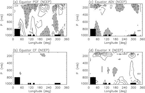
Fig. 11 Schematic depiction of the vertical structure of tropical atmosphere for (upper) CQE’s 2-phase view, and (lower) observed 4-phase structure. The types of convection are represented by the clouds, while the corresponding profiles of saturation moist static energy anomaly are plotted underneath them (adapted from Lin et al., Citation2015).
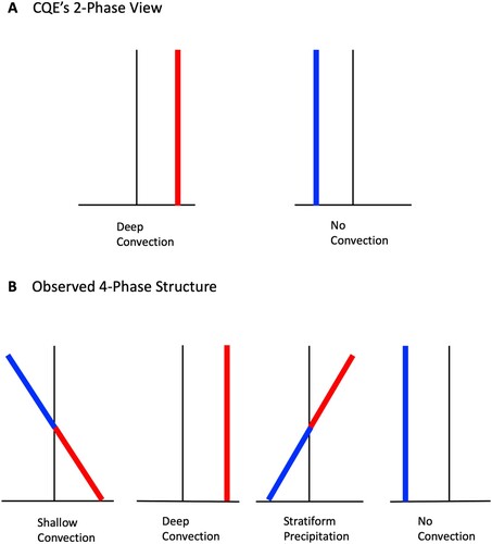
Fig. 12 Schematic of the IFS mass flux convection scheme.
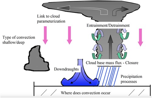
Fig. 13 24–48 h convective and stratiform rainfall (mm day−1) over North America for May 2002 with the operational IFS in 2002 (left column) and with the revised convective initiation allowing convection to depart from any model layer below 350 hPa (right column). This version became operational in 2003.
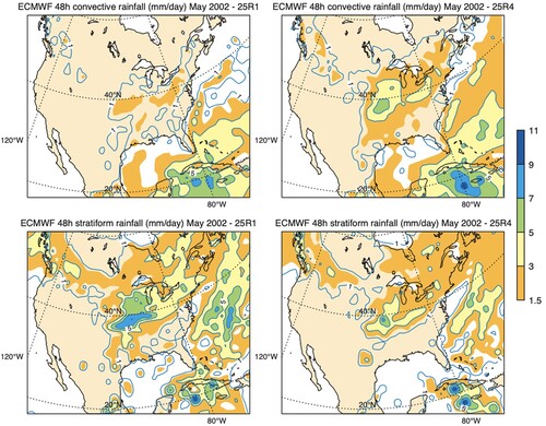
Fig. 14 Wavenumber frequency spectra of the outgoing longwave radiation from NOAA data (a) and from multi-year integrations with the IFS using the operational cycle in 2006 (b) and with the version that became operational in 2008 (c); the MJO spectral band is highlighted by the black rectangle. (d)–(e) measure the gain in prediction skill: (d) evolution of the prediction skill of the IFS for the MJO between 2002 and 2013 as given by the bivariate correlation with the observed empirical orthogonal functions for wind and outgoing longwave radiation, a value of 0.6 (red line) delimits skillfull forecasts (Vitart & Molteni, Citation2010), (e) statistics of cyclone positions errors (km) as a function of forecast lead time from the 40 km resolution forecasts in 2005/6 (blue), the 25 km forecasts in 2006/7 (red) and the 25 km forecasts in 2008 (green).
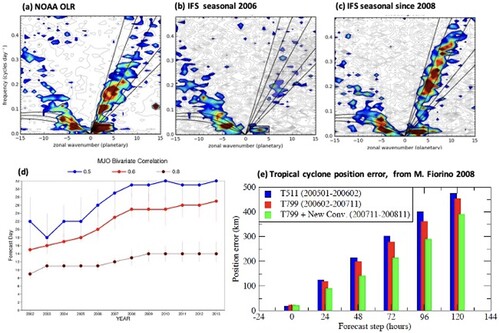
Fig. 15 Composite diurnal cycle of precipitation (mm day−1) during JJA 2013 over Europe and continental United States from radar observations (black) and from 24 to 48 h reforecasts with the IFS operational cycle in 2012 (sky blue) and the operational cycle in 2013 (red).
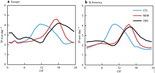
Fig. 16 Cloud and radiation evaluation from multi-annual coupled integrations with the IFS Cy47r1. (a)–(b) difference in top of atmosphere net shortwave radiation (W/m2) between the model and the Earth’s Radiant Energy System (CERES) Energy Balanced and Filled (EBAF) product for (a) the operational model version in 2018 and (b) as (a) but with all the changes relating to the mixed phase microphysics added during 2016–2018 removed.
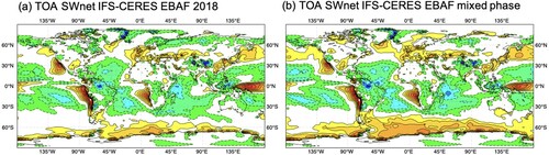
Fig. 17 Evolution of continental convective systems over tropical Africa during 12 September 2017 in 3-hourly slots from 15 to 21 UTC as seen by Meteosat-11 infrared image at 10.9 μ wavelength (a,b,c), as well as 3 hourly accumulated rainfall (mm) from 12 to 15, 15 to 18 and 18 to 21 UTC from the TRMM 3B42 product (d,e,f), from the 4 km IFS reforecasts with (g,h,i) (operational version) and without (j,k,l) the deep convection scheme, and with the revised deep convective closure (m,n,o). The IFS reforecasts start at 11 September 2017 at 00 UTC and use the model cycle operational in 2019. There is no TRMM 3B42 data East of 25°E at 21 UTC.
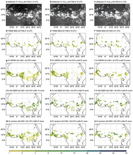
Fig. 18 Fraction of the resolved precipitation compared to the total precipitation. The 6-hourly model areal mean precipitation rates are averaged for each experiment over the 15 runs.
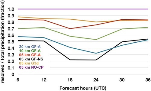
Fig. 19 As in except for Root Mean Square Error (RMSE) and mean error (Bias). Units are mm/6hr.
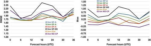
Fig. 20 6hr precipitation forecasts from the HRRR (middle and right panel) for runs without convective parameterizations (middle) and runs with the GF scheme (right panel), compared to observations (right panel) for the same period.
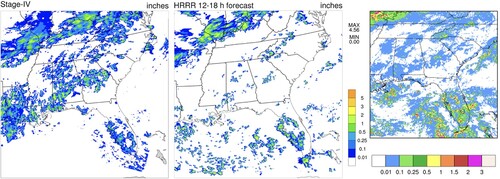
Fig. 21 Frequency BIAS ration for 12hr accumulated precip, August 8–9, a HRRR run without convective parameterizations (blue) and with a version of the GF scheme (red) in dependence of threshold precipitation amounts over the 12 h period ending on August 9, 00z.
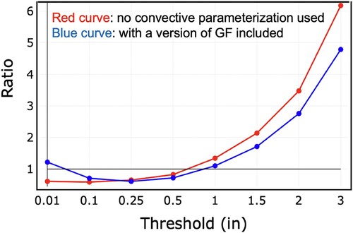
Fig. 22 A Comparison of deep, congestus (mid), and shallow convection massflux profiles for Single Column Model simulations (left) and radar observations (right) during the TWP-ICE field experiment. Observations are from Kumar et al. (Citation2015) showing mass flux profiles derived from windprofilers (black) and CPOL data (red).
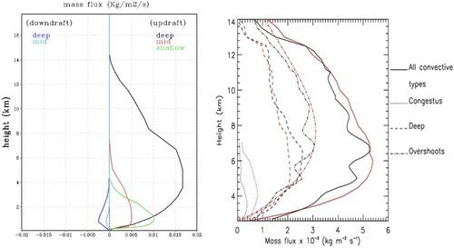
Fig. 23 The time average of the diurnal cycle of the grid-scale vertical moistening (panels A and B) and heating (panels C and D) tendencies associated with the three parameterized convective modes (shaded). The total precipitation and the GF parameterized precipitation from the deep and congestus plumes are shown by the graphic lines: black, green, and purple, respectively. The upper rows show model results without Bechtold’s closure, while in the lower row, this closure is applied (see text for further details).
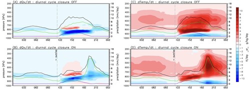
Fig. 24 Scatter plot of the CAPE change due to the ambient virtual temperature change vs. CAPE change due to large-scale forcing from advection and radiative cooling during the ARM summer 1997 IOP. Triangles are for convective periods, crosses and dots are for non-convective periods, the latter of which are for CIN < −100 J/kg. From Zhang (Citation2002).
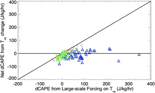
Fig. 25 Precipitation time series observed (blue line) during the ARM 1997 IOP at the SGP site and simulated by a single column model using the original ZM scheme (dashed line, top) and the revised ZM scheme with dCAPE closure (dashed line, bottom).
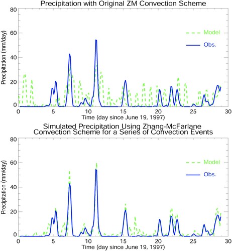
Fig. 26 Schematic showing the microphysical processes represented in the convective microphysics parameterization of the ZM scheme.
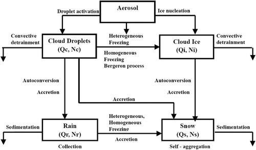
Fig. 27 (a) Frequency distributions of precipitation rate and (b) cumulative contribution from each binned precipitation rate based on daily mean precipitation data. The results are for the global belt of 20°S–20°N from the Tropical Rainfall Measurement Mission (TRMM) observation (black line), CTL (blue line) and EXP (red line). From Wang et al. (Citation2016).
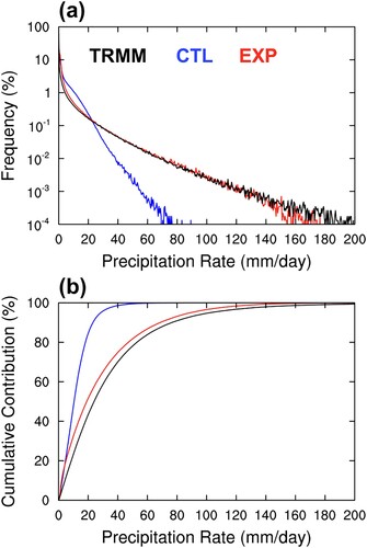
Fig. 28 Virtual potential temperatures for fractional mixtures of updraft and environmental air, where and
denote the fraction where the mixture is just saturated and just buoyant with respect to the environment.
is the virtual potential temperature of the mixture that is just saturated.
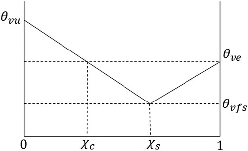
Fig. 29 Schematic vertical structure and physical processes of the stratocumulus topped boundary layer.
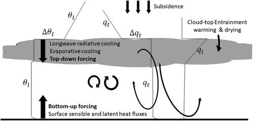
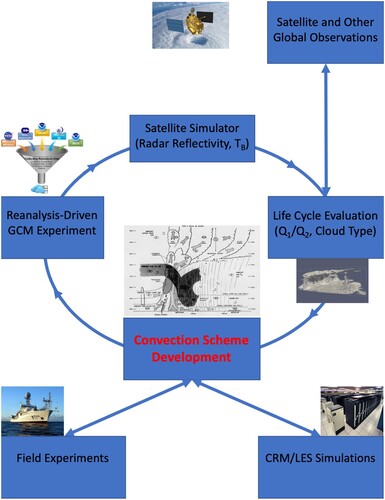
Fig. 30 Proposed strategy for convection scheme development. Schematic of convective system is from Zipser (Citation1977). Photos courtesy of NASA and NOAA.