Figures & data
Fig. 1 (a) Map of the product of the differences of 20-year averaged land surface air temperature anomalies, centered at the extrema of global mean oscillation (inset): [(1900-1920)–(1935-1955)]×[(1935-1955)–(1970-1990)] (from Schlesinger & Ramankutty, Citation1994). (b) AMO index (upper) and its correlation with SST anomalies (lower) (from Enfield et al., Citation2001).
![Fig. 1 (a) Map of the product of the differences of 20-year averaged land surface air temperature anomalies, centered at the extrema of global mean oscillation (inset): [(1900-1920)–(1935-1955)]×[(1935-1955)–(1970-1990)] (from Schlesinger & Ramankutty, Citation1994). (b) AMO index (upper) and its correlation with SST anomalies (lower) (from Enfield et al., Citation2001).](/cms/asset/735781c2-dbb2-4775-9f4b-d464f9d0b8ef/tato_a_2086847_f0001_oc.jpg)
Fig. 2 (a) Schematic of the Atlantic meridional overturning circulation (from Wust Citation1936 ). (b) Schematic of the vertical structure of global thermohaline circulation (from Gordon, Citation1991). (c) Schematic of the horizontal structure of global thermohaline circulation (from Rahmstorf, Citation2006).
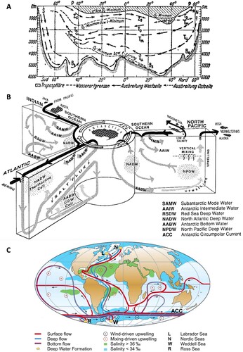
Fig. 3 Schematic of the existing THC theories and AMO theories. Numbers in parentheses denote that the process is involved in corresponding AMO theories: (1) stochastic forcing theory, (2) NAO coupled oscillator, (3) zonal-meridional oscillator, (4) delayed advective oscillator, (5) ice coupled oscillator, (6) cloud-radiation feedback theory, and (7) aerosol forcing theory.
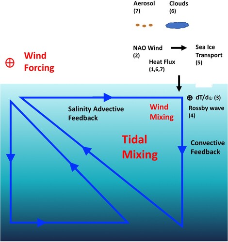
Fig. 4 Regression of Atlantic basin zonal mean (a) temperature, and (b) salinity to THC index at lag +10 years (from Delworth et al., Citation1993). Regression of SST (shaded), SLP (contours), and surface winds (vectors) to the AMO index for (c) fully coupled models, and (d) slab-ocean models (from Clement et al., Citation2015). Differences between warm and cold AMO phases for (e) aerosol burden, and (f) surface net shortwave flux (from Booth et al., Citation2012).
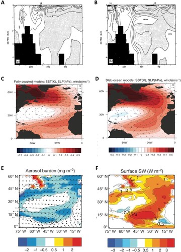
Fig. 5 Maximum entropy spectra of (a) North Atlantic Ocean SST, (b) Nino3.4 SST, and (c) global mean surface temperature from LMR reanalysis, and (d) AMOC index from Mjell et al. (Citation2016), (e) solar forcing from IPCC AR6, (f) volcano forcing from IPCC AR6, and (g) tidal gravitational forcing from NASA JPL. All data are for the past 2000 years.
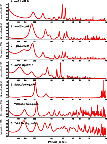
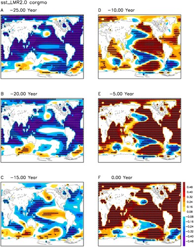
Fig. 6 Lag-correlation of 40–100-year filtered LMR reanalysis SST anomaly with AMO index for lag (a) -25 years, (b) -20 years, (c) -15 years, (d) -10 years, (e) -5 years, and (f) 0 year. Stars denote the grids with correlation coefficients above the 95% confidence level.
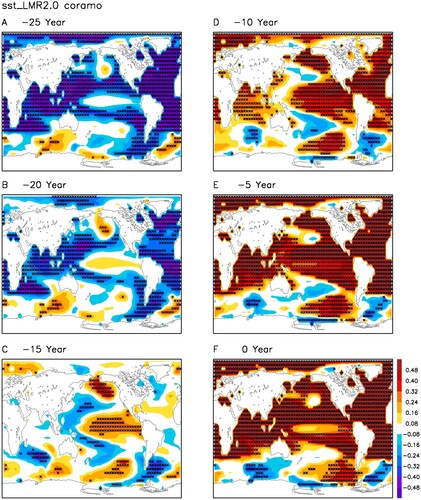
Fig. 7 Lag-correlation of 40–100-year filtered LMR reanalysis SST anomaly with AMOC index from Mjell et al. (Citation2016) for lag (a) -15 years, (b) -10 years, (c) -5 years, (d) 0 year, (e) +5 years, and (f) +10 years. Stars denote the grids with correlation coefficients above the 95% confidence level.
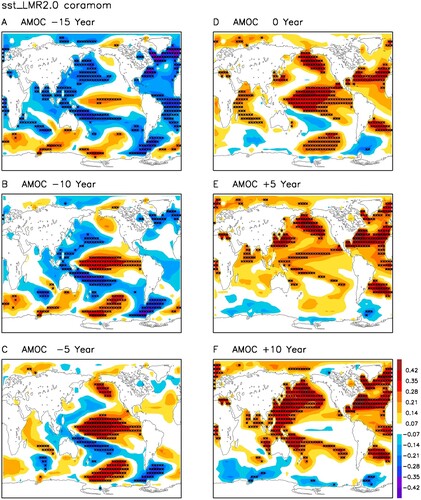
Fig. 8 Lag-correlation of 40–100-year filtered LMR reanalysis SST anomaly with volcano forcing from IPCC AR6 for lag (a) 0 year, (b) +5 years, (c) +10 years. Lag-correlation of 40–100-year filtered LMR reanalysis surface downward shortwave flux anomaly with AMO index for lag (d) -10 years, (e) -5 years, (f) 0 year. Stars denote the grids with correlation coefficients above the 95% confidence level.
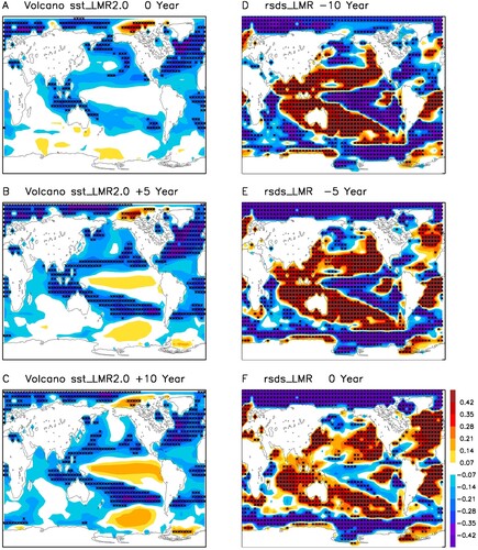
Fig. 9 Lag-correlation of 40–100-year filtered LMR reanalysis SST anomaly with tidal gravitational forcing from NASA JPL for lag (a) -15 years, (b) -10 years, (c) -5 years, (d) 0 year, (e) +5 years, and (f) +10 years. Stars denote the grids with correlation coefficients above the 95% confidence level.
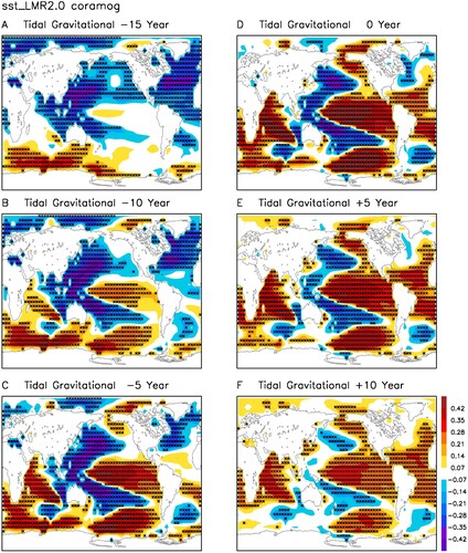
Fig. 10 Schematic depiction of the structure and physical mechanisms of the AMO.
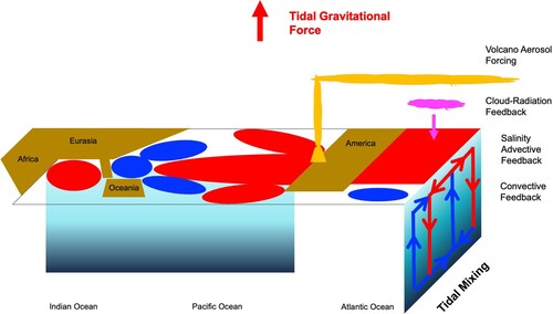
Fig. 11 Correlation of AMO index with (a) sea level pressure and (b) surface air temperature for NOAA 20C reanalysis (1871-2008). Shading denotes regions with correlation above 95% confidence level (from Alexander et al., Citation2014). (c) Regression of JAAS precipitation in Africa and India to AMO index for 1900–2002 (from Zhang & Delworth, Citation2006). (d) Regression of JJA precipitation in Asia to AMO index for 1900-2002. Green contour denotes regions above 95% confidence level (from Wang et al., Citation2009).
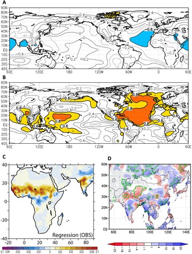
Fig. 12 (a) Annual mean pressure vertical velocity anomaly (Pa/s) at 500 mb over the tropical Pacific; negative values indicate upward motion. (b) Annual mean ocean temperature anomaly (K) across 10°S in the tropical Pacific. (c) Same as in (b), but across 170°E in the tropical Pacific. (d) Annual mean zonal ocean current anomaly (m/s) across 170°E in the tropical Pacific. (e) Schematic diagram of global tropical responses to the North Atlantic freshwater forcing and the mechanism. The blue circle over the Central American coast emphasizes the important region of atmospheric linkage between the Atlantic and Pacific. The anomalous surface zonal wind over the northern tropical Pacific strengthens the trade wind there, while over the southern tropical Pacific, it weakens the trade wind. (f) Anomalous summer precipitation (m/yr) and flow at 925 mb over the Indian and eastern China regions. (from Zhang & Delworth, Citation2005).
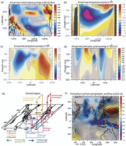
Fig. 13 Lag-correlation of 40–100-year filtered LMR reanalysis SLP anomaly with AMO index for lag (a) -30 years, (b) -15 years, and (c) 0 year. Lag-correlation of 40–100-year filtered LMR reanalysis Z500 with AMO index for lag (d) -30 years, (e) -15 years, and (f) 0 year. Stars denote the grids with correlation coefficients above the 95% confidence level.
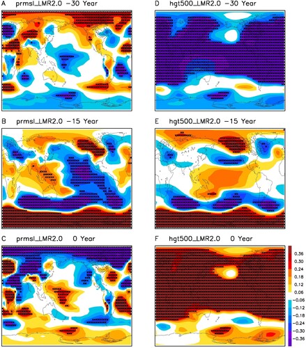
Fig. 14 Lag-correlation of 40–100-year filtered LMR reanalysis land surface air temperature anomaly with AMO index for lag (a) -30 years, (b) -20 years, (c) -10 years, (d) 0 year, (e) +10 years, and (f) +20 years. Stars denote the grids with correlation coefficients above the 95% confidence level.
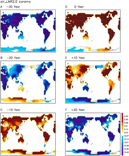
Fig. 15 Lag-correlation of 40–100-year filtered LMR reanalysis PDSI anomaly with AMO index for lag (a) -30 years, (b) -20 years, (c) -10 years, (d) 0 year, (e) +10 years, and (f) +20 years. Stars denote the grids with correlation coefficients above the 95% confidence level.
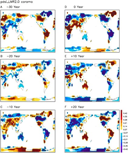
Fig. 16 Schematic depiction of the global impacts of AMO. Red (blue) shading denotes the region with statistically significant surface air temperature (PDSI) anomalies. The phase lag to the AMO index is represented by the arrows. The phase clock is also shown.
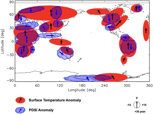
Fig. 17 (A) Observed (HadCRUT4.6, NOAAGlobalTemp) and CMIP6 model global mean surface temperature change for 1850-2020. Shading shows ±1 standard deviation about the ensemble mean (from Modak & Mauritsen, Citation2021). (B) Observed temperature anomalies for the past 2000 years from seven paleoclimate reconstruction methods together with CMIP5 models subjected to 30–200 yr bandpass filters (from PAGES Citation2k Consortium, Citation2019). (C) Maximum entropy spectra of observed global mean surface temperature from three datasets for 1880-2016.
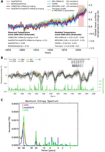
Fig. 18 Lag-correlation of 40–100-year filtered LMR reanalysis SST anomaly with global mean surface temperature anomaly for lag (a) -25 years, (b) -20 years, (c) -15 years, (d) -10 years, (e) -5 years, and (f) 0 year. Stars denote the grids with correlation coefficients above the 95% confidence level.