New HEAVY Models for Fat-Tailed Realized Covariances and Returns

Figures & data

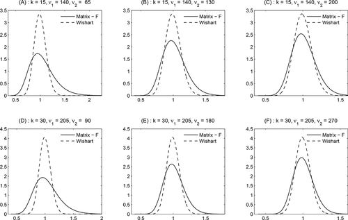
Figure 1. The rescaled matrix-F and the Wishart distribution. This figure shows pdfs associated with a matrix-F distribution with ν₁ and ν₂ degrees of freedom and a Wishart distribution with ν₁ degrees of freedom for a k × k matrix RC_t . We plot the pdf of one of the main-diagonal entries RC _{ii, t} (i = 1, …k), for k = 15 (upper panels) and k = 30 (lower panels) for various degrees of freedom. The solid line corresponds with the F distribution, while the dashed line represents the Wishart (χ²) distribution.

Table 1. Parameter estimations of HEAVY GAS DGP. This table shows Monte Carlo averages and standard deviations (in parentheses) of parameter estimates from simulated HEAVY GAS processes. The table reports the mean and the standard deviation in parentheses based on 1000 replications

		k = 5			k = 15
Coef.	True	T = 500	T = 1000	True	T = 500	T = 1000
α	0.80	0.797 (0.036)	0.798 (0.025)	0.80	0.801 (0.022)	0.800 (0.016)
β	0.97	0.966 (0.005)	0.968 (0.004)	0.97	0.966 (0.002)	0.968 (0.001)
ν0	12.00	12.419 (2.233)	12.179 (1.460)	12.00	12.097 (1.195)	12.054 (0.803)
ν1	22.00	22.063 (0.794)	22.037 (0.559)	140.00	140.57 (4.025)	140.28 (2.829)
ν2	35.00	35.127 (2.049)	35.054 (1.435)	65.00	65.030 (0.813)	64.998 (0.588)
		k = 30			k = 50
α	0.80	0.799 (0.010)	0.799 (0.007)	0.80	0.799 (0.005)	0.799 (0.004)
β	0.97	0.966 (0.001)	0.968 (0.001)	0.97	0.967 (0.001)	0.969 (0.000)
ν0	12.00	12.083 (0.857)	12.046 (0.610)	12.00	12.096 (0.757)	12.059 (0.545)
ν1	205.00	205.72 (2.605)	205.29 (1.825)	300.00	300.82 (2.152)	300.35 (1.464)
ν2	90.00	90.025 (0.473)	90.020 (0.346)	150.00	150.01 (0.497)	150.00 (0.343)

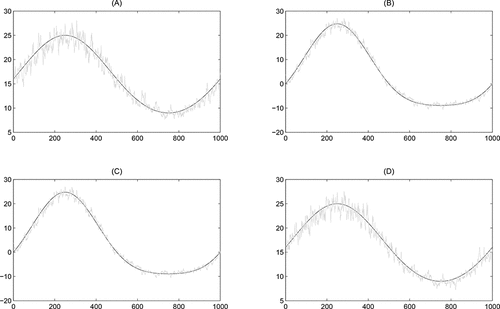
Figure 2. Model fit for a deterministic DGP. This figure shows a realization of the simulated (co)variance process of (15(15) $$\begin{array}{ccc}\hfill y_t|{\mathcal{F}}_{t-1}& \sim & t({\nu }_0,V_t),R{C}_t|{\mathcal{F}}_{t-1}\sim F({\nu }_1,{\nu }_2,V_t),\hfill \\ \hfill V_t& =& \bar{V}+\gamma V_{t-1}+{\eta }_t,{\eta }_t\sim F({\nu }_{\eta ,1},{\nu }_{\eta ,2},V_{0,\eta }),\hfill \\ \hfill V_0& =& 4\left(\begin{array}{cc}\hfill 1& \hfill 0.7\\ \hfill 0.7& \hfill 1\end{array}\right),\hfill \end{array}$$(15) ) (black line) with T = 1000 and the fit from the HEAVY GAS tF model (gray line). Panels A and D represent the volatilities, while panels B and C present the correlation and covariance, respectively.

Table 2. Statistical fit on stochastic DGP. This table shows Monte Carlo averages and standard deviations (in parentheses) of the RMSE defined in (17(17) $$\begin{array}{ccc}\hfill \text{RMSE}& =& {\left[\frac{1}{T}\sum _{t=1}^T{\parallel V_t-{\widehat{V}}_t\parallel }^2\right]}^{1/2}\hfill \\ & =& {\left[\frac{1}{T}\sum _{i,j,t}{(V_{ij,t}-{\widehat{V}}_{ij,t})}^2\right]}^{1/2},\hfill \end{array}$$(17) ) over all simulation paths of three misspecified models with respect to the true bivariate covariance matrix, which is simulated from the SV process of (15(15) $$\begin{array}{ccc}\hfill y_t|{\mathcal{F}}_{t-1}& \sim & t({\nu }_0,V_t),R{C}_t|{\mathcal{F}}_{t-1}\sim F({\nu }_1,{\nu }_2,V_t),\hfill \\ \hfill V_t& =& \bar{V}+\gamma V_{t-1}+{\eta }_t,{\eta }_t\sim F({\nu }_{\eta ,1},{\nu }_{\eta ,2},V_{0,\eta }),\hfill \\ \hfill V_0& =& 4\left(\begin{array}{cc}\hfill 1& \hfill 0.7\\ \hfill 0.7& \hfill 1\end{array}\right),\hfill \end{array}$$(15) ). We compare the HEAVY GAS tF model with the HJK model and the CAW model. The table reports the mean and the standard deviation of the mean in parentheses based on 1500 simulation paths

	HGAS tF	HJK	CAW
mean	11.42	12.66	13.49
st. dev.	(0.14)	(0.17)	(0.18)

Table 3. Kolmogorov–Smirnov test on the distribution of realized variances. This table shows p-values associated with the Kolmogorov–Smirnov test on realized variances of 30 equities. The columns represent the Ticker symbol as well as p-values corresponding with the null hypothesis that RC_t is χ² or F distributed

Ticker	H0: χ^2	H0: F	Ticker	χ^2	F	Ticker	χ^2	F
AA	0.00	0.05	MCD	0.00	0.01	BHI	0.00	0.82
AXP	0.00	0.00	PFE	0.00	0.86	BAC	0.00	0.00
BA	0.00	0.20	PG	0.00	0.22	C	0.00	0.00
CAT	0.00	0.44	WMT	0.00	0.25	DD	0.00	0.11
GE	0.00	0.05	XOM	0.00	0.84	DOV	0.00	0.93
HD	0.00	0.23	AIG	0.00	0.01	DUK	0.00	0.17
HON	0.00	0.19	AEP	0.00	0.48	F	0.00	0.06
IBM	0.00	0.06	ABT	0.00	0.86	JNJ	0.00	0.11
JPM	0.00	0.05	AEE	0.00	0.05	KEY	0.00	0.46
KO	0.00	0.15	BAX	0.00	0.87	LLY	0.00	0.97

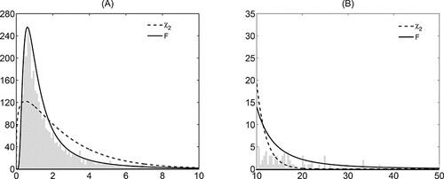
Figure 3. The fit of the probability distribution of the realized variance of BA. This figure shows a histogram of the realized variances (RV) of Boeing over the period 2001–2014. Panel A shows the histogram for $\text{RV}<10$, while panel B shows the remaining part of the histogram for values of RV larger than 10. The solid and dashed curves present the best-fitting F and χ² distribution, respectively.

Table 4. Parameter estimates, likelihoods, and information criteria. This table reports maximum likelihood parameter estimates of the HEAVY GAS (HAR) tF model, the IW-A model of Jin and Maheu (2016), the HJK model of Hansen, Janus, and Koopman (2016), and the CAW model of Golosnoy, Gribisch, and Liesenfeld (2012), applied to daily equity returns and/or daily realized covariances. Panels A.1 and A.2 list results for two randomly chosen sets containing five different assets. Panel B considers 15 assets and panel C shows the results for the full set of 30 assets. Standard errors are provided in parentheses. We report the total likelihood ${\mathcal{L}}^{*}$ and the BIC (in thousands) of the IW-A and the CAW model and the likelihood associated with the realized covariance matrix (i.e., the matrix-F and the Wishart distributions) for the GAS models. Data are observed over the period January 2, 2001 until July 31, 2014 (T = 3415 trading days)

	α	β(β1)	β2	β3	ν0	ν1(ν IW )	ν2	${\mathcal{L}}^{*}$	BIC
Panel A.1: BA/HD/JPM/PFE/PG
GAS tF	0.859	0.989			10.09	69.86	35.26	−11,906	23.85
	(0.017)	(0.000)			(0.615)	(1.429)	(0.414)
GAS-H tF	0.963	0.869	0.083	0.042	10.37	70.87	35.90	−11,387	22.82
	(0.018)	(0.006)	(0.007)	(0.003)	(0.652)	(1.339)	(0.398)
HJK	0.054	0.965				17.83		−21,529	43.10
	(0.001)	(0.001)				(0.099)
CAW	0.336	0.647				19.74		−18,030	36.08
	(0.005)	(0.005)				(0.111)
IW-A		0.379	0.400	0.194		22.89		−13,104	26.24
		(0.005)	(0.007)	(0.006)		(0.105)
Panel A.2: CAT/HON/IBM/MCD/WMT
GAS tF	0.826	0.990			10.33	72.54	34.53	−4828	9.70
	(0.020)	(0.000)			(0.643)	(1.999)	(0.438)
GAS-H tF	0.931	0.878	0.075	0.041	10.58	72.85	35.17	−4387	8.81
	(0.019)	(0.006)	(0.007)	(0.003)	(0.673)	(1.579)	(0.417)
HJK	0.044	0.975				18.97		−12,324	24.69
	(0.001)	(0.001)				(0.106)
CAW	0.313	0.670				20.26		−10,046	20.12
	(0.005)	(0.005)				(0.115)
IW-A		0.338	0.442	0.190		23.05		−5552	11.14
		(0.005)	(0.007)	(0.006)		(0.107)
Panel B: AA/AXP/BA/CAT/GE/HD/HON/IBM/JPM/KO/MCD/PFE/PG/WMT/XOM
GAS tF	0.666	0.993			12.69	140.3	64.26	149,088	−298.1
	(0.005)	(0.000)			(0.506)	(0.802)	(0.218)
GAS-H tF	0.784	0.883	0.070	0.043	12.97	141.9	65.06	152,279	−304.4
	(0.006)	(0.002)	(0.003)	(0.001)	(0.519)	(0.790)	(0.221)
HJK	0.026	0.979				37.47		88,987	−177.9
	(0.000)	(0.000)				(0.070)
CAW	0.235	0.753				39.32		104,666	−209.3
	(0.001)	(0.001)				(0.074)
IW-A		0.246	0.467	0.257		44.40		139,138	−278.2
		(0.002)	(0.003)	(0.003)		(0.062)
Panel C: All equities (k = 30)
GAS tF	0.520	0.997			12.65	203.8	91.71	937,986	−1876
	(0.002)	(0.000)			(0.407)	(0.430)	(0.161)
GAS-H tF	0.648	0.891	0.065	0.042	13.03	204.8	92.78	948,944	−1898
	(0.002)	(0.001)	(0.002)	(0.001)	(0.383)	(0.417)	(0.131)
CAW	0.173	0.821				57.04		725,787	−1452
	(0.001)	(0.001)				(0.050)
IW-A		0.180	0.468	0.332		66.07		883,287	−1767
		(0.001)	(0.002)	(0.001)		(0.038)

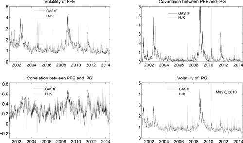
Figure 4. Estimated volatilities and correlations. This figure depicts estimated volatilities of PFE and PG at the main diagonal and their pairwise correlations and covariances at the off-diagonal, estimated by the HEAVY GAS tF and HJK model. The black line corresponds with the HEAVY GAS tF model, while the gray line denotes the fit from the HJK model. The estimation is based on the full sample, which runs from January 2, 2001, until July 31, 2014 (3415 observations).

Table 5. Out-of-sample log-scores and ex post conditional standard deviations. This table shows the mean of log scores, defined in (21(21) $$\begin{array}{c}\hfill S_{ls,t}(X_t,M_j)=log{p}_t\left(X_t\right|V_t,{\mathcal{F}}_{t-1},M_j),\end{array}$$(21) ) and ex post portfolio standard deviation, based on one-step ahead predictions of the covariance matrix, according to the HEAVY (HAR) GAS tF, HJK, CAW, IW-A, and the EWMA model for two pairs of five assets (panel A), one pair of 15 assets (panel B) and for all equities (panel C, k = 30). The highest (lowest) value of the predictive log-score (portfolio standard deviation) across the models are marked bold. In addition, we report HAC-based test-statistics on the difference in predictive ability (${\text{DM}}_{\text{DF}}$) and portfolio standard deviation $\left({\text{DM}}_{{\sigma }_p}\right)$ between the HEAVY GAS HAR tF model and the other considered models. The superscripts *^**, **, and * indicate significance at the 1%, 5%, and 10% level, respectively. The out-of-sample period goes from 2007 until July 2014 and contains 1914 observations

	GAS HAR tF	GAS tF	HJK	CAW	IW-A	EWMA	BEKK-t
Panel A: BA/HD/JPM/PFE/PG
S^ls (RCt )	–2.11	–2.23	–6.22	–4.44	–2.72	–4.47	–9.08
${\text{DM}}_{\text{DF}}$		(3.13)^***	(6.72)^***	(3.61)^***	(4.50)^***	(11.90)^***	(21.18)^***
S^ls (yt )	–7.30	–7.31	–7.49	–7.31	–7.32	–7.37	–7.40
${\text{DM}}_{\text{DF}}$		(2.59)^***	(8.77)^***	(1.37)	(2.86)^***	(6.96)^***	(5.70)^***
σ p	0.790	0.791	0.810	0.794	0.794	0.797	0.824
${\text{DM}}_{{\sigma }_p}$		(–6.00)^***	(–5.81)^***	(–3.73)^***	(–3.08)^***	(–4.82)^***	(–16.41)^***
Panel B: k = 15
S^ls (RCt )	58.28	57.52	34.62	42.03	53.86	49.08	5.96
${\text{DM}}_{\text{DF}}$		(3.68)^***	(11.51)^***	(8.28)^***	(4.45)^***	(11.85)^***	(20.92)^***
S^ls (yt )	–19.95	–19.98	–20.54	–19.99	–20.09	–20.07	–20.30
${\text{DM}}_{\text{DF}}$		(5.33)^***	(14.50)^***	(3.42)^***	(7.35)^***	(7.17)^***	(9.45)^***
σ p	0.629	0.630	0.648	0.632	0.632	0.637	0.695
${\text{DM}}_{{\sigma }_p}$		(–6.00)^***	(–5.81)^***	(–3.73)^***	(–3.08)^***	(–4.82)^***	(–16.41)^***
Panel C: All equities (k = 30)
S^ls (RCt )	316.48	313.39		238.97	294.60	292.20	109.08
${\text{DM}}_{\text{DF}}$		(5.08)^***		(16.73)^***	(7.45)^***	(12.93)^***	(26.59)^***
S^ls (yt )	–40.74	–40.82		–40.74	–40.94	–40.78	–41.87
${\text{DM}}_{\text{DF}}$		(8.17)^***		(0.08)	(4.75)^***	(1.20)	(16.75)^***
σ p	0.571	0.572		0.574	0.574	0.579	0.654
${\text{DM}}_{{\sigma }_p}$		(–3.83)^***		(–3.58)^***	(–3.34)^***	(–8.72)^***	(–18.45)^***

——— (2016), “Bayesian Semiparametric Modeling of Realized Covariance Matrices,” Journal of Econometrics , 192, 19–39.

 Web of Science ®Google Scholar

Hansen, P. , Janus, P. , and Koopman, S. (2016), “Realized Wishart-GARCH: A Score-driven Multi-Asset Volatility Model,” TI 2016-061/III, Tinbergen Institute Discussion Paper.

 Google Scholar

Golosnoy, V. , Gribisch, B. , and Liesenfeld, R. (2012), “The Conditional Autoregressive Wishart Model for Multivariate Stock Market Volatility,” Journal of Econometrics , 167, 211–223.

 Web of Science ®Google Scholar