Mean-Structure and Autocorrelation Consistent Covariance Matrix Estimation

Figures & data

Table 1 A summary of the robust estimators introduced in Section 2.4, where AC, CV, J, W, and WZ represent estimators proposed in Altissimoa and Corradic (2003), Crainiceanu and Vogelsang (2007), Jirak (2015), Wu (2004), and Wu and Zhao (2007), respectively.

	Robustness		Generality & optimality
Estimators	(a) J change points	(b) Continuous trend	(c) Dimension d	(d) Optimal $\mathcal{l}$
AC	Yes, $J<\infty$	No	d = 1	Not derived
CV, J	Yes, J = 1	No	d = 1	Not derived
W, WZ	No	Yes	d = 1	Not derived
${\widehat{\mathbf{\Sigma }}}_{0,2,n}$ (proposal)	Yes, $J=o(n^{1/5})$	Yes	$d\ge 1$	Derived

NOTE: The last row shows a special case of our proposed estimator ${\widehat{\mathbf{\Sigma }}}_{p,q,n}$, which will be defined in (8). Note that (a) states the robustness against piecewise-constant means with J CPs. Note also that three estimators (namely WZ1, WZ2, and WZ3) are proposed in WZ, but they share the same facts (a)–(d).

Table 2 Summary of the statistical meanings of p, q, P and their associated quantities.

Order	Related quantity	Statistical meaning
p	${\mathbf{\Sigma }}_p=\sum _{k\in \mathbb{Z}}|k{|}^p{\mathbf{\Pi }}_k$	The estimand is ${\mathbf{\Sigma }}_p$. If p = 0, ${\mathbf{\Sigma }}_0\equiv \mathbf{\Sigma }$ reduces to the ACM (1).
q	$K_q(t)=(1-|t{|}^q)1(\left|t\right|\le 1)$	The qth order kernel $K_q(·)$ is used in the estimator ${\widehat{\mathbf{\Sigma }}}_{p,q,n}$.
$P\equiv p+q$	${\mathbf{\Upsilon }}_P=\sum _{k\in \mathbb{Z}}\left|k{|}^P\right|{\mathbf{\Pi }}_k|$	If ${\mathbf{\Upsilon }}_P$ is finite with a larger P, then the autocorrelation is weaker.

Fig. 1 (a) A typical realization of the time series with the mean function defined in (21). (b) The density functions of ${\widehat{\Sigma }}_{0,2,n}$ and ${\widehat{\Sigma }}_{\text{QS},n}$ when n = 400. The true value is Σ = 9.

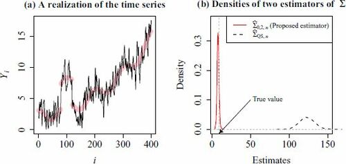
Fig. 2 The values of $\text{log}\hspace{0.17em}({\text{MSE}}_0)$ and $\text{log}\hspace{0.17em}({\text{MSE}}_{\text{sd}})$ are plotted against n, where ${\text{MSE}}_0$ denotes the MSE when the jump size ξ = 0, and ${\text{MSE}}_{\text{sd}}$ denotes the standard deviation of the MSEs across different ξ. Recall that smaller ${\text{MSE}}_0$ and smaller ${\text{MSE}}_{\text{sd}}$ imply higher efficiency and robustness, respectively. Note that ${\widehat{\sigma }}_{\text{AC},n}^2$ is computed only when $n\le 400$ because it requires a computationally intensive cross-validation step. Note that horizontal axis is plotted in the logarithmic scale for better visualization.

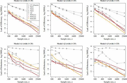
Fig. 3 Thin solid line: A realization of $\left\{Y_i\right\}$ in Model A2 of length n = 400. Thick solid line: The nonconstant mean function $\left\{{\mu }_i\right\}$ in Section 5.2. Dotted vertical lines: The change points.

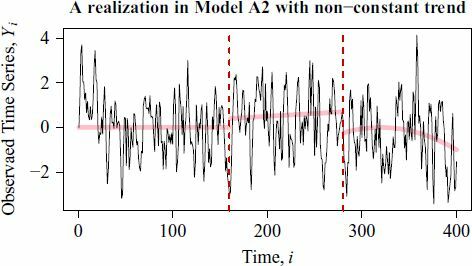
Fig. 4 The values of $\text{log}\hspace{0.17em}\left\{\text{MSE}(·)\right\}$ of different estimators are plotted against the sample size n in Models A1–A3. Here the mean function consists of nonconstant trends and multiple jumps (see Section 5.2 and Figure 3). Note that horizontal axis is plotted in the logarithmic scale.

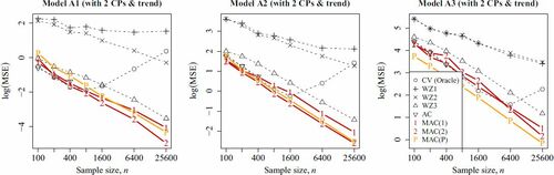
Fig. 5 The values of $\text{log}\hspace{0.17em}\left\{{\text{MSE}}_{\mathit{W}}(·)\right\}$ for ${\widehat{\mathbf{\Sigma }}}_{\text{Bart},n}$, ${\widehat{\mathbf{\Sigma }}}_{\text{QS},n},{\widehat{\mathbf{\Sigma }}}_{0,1,n}^{‡}$, ${\widehat{\mathbf{\Sigma }}}_{0,2,n}^{‡}$ and ${\widehat{\mathbf{\Sigma }}}_{0,2,n}^{†}$ in the heteroscedastic case are plotted against n, where $\text{vec}(\mathit{W})={(1,1/2,1/2,1)}^{⊺}$ is used, and ${\text{MSE}}_{\mathit{W}}(·)$ is defined in (16). The left and right plots show the results in the constant mean and nonconstant mean cases, respectively. Note that the horizontal axes are plotted in the logarithmic scale.

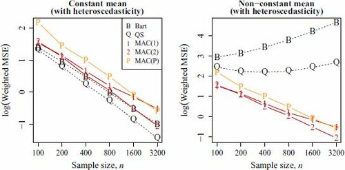
Fig. 6 The powers of the CP tests defined in Section 5.4 are plotted against the jump magnitude ξ under Model B2. The scenarios under well-specified alternative H₁ and misspecified alternative $H_1^{\prime }$ are shown in the upper and lower plots, respectively. Dashed horizontal lines indicate the significance level $\alpha =5\%$ and zero. Note that horizontal axis is plotted in the logarithmic scale for better visualization.

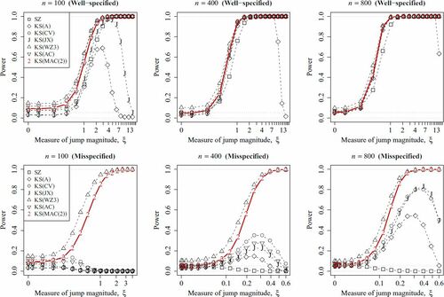
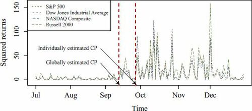
Fig. 7 Time series plot of $\left\{Y_i\right\}$, that is, the daily S&P 500 Index (3 January 2006–30 December 2011) in the log scale (see Section 6.1). The vertical dotted line indicates the value of ${\widehat{D}}_{\text{WZ}}$ estimated by the statistic in Wu and Zhao (2007). Here ${\sigma }^2$ is estimated by MAC(2).

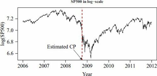
Fig. 8 The squared returns of four stock indices (1 July 2008–30 December 2008) (see Section 6.2). The two vertical lines denote the CP locations. The earlier and later CPs are detected by the multivariate and univariate CUSUM CP estimators, respectively.

Altissimoa, F., and Corradic, V. (2003), “Strong Rules for Detecting the Number of Breaks in a Time Series,” Journal of Econometrics, 117, 207–244. DOI: https://doi.org/10.1016/S0304-4076(03)00147-7.

 Web of Science ®Google Scholar

Crainiceanu, C. M., and Vogelsang, T. J. (2007), “Nonmonotonic Power for Tests of a Mean Shift in a Time Series,” Journal of Statistical Computation and Simulation, 77, 457–476. DOI: https://doi.org/10.1080/10629360600569394.

 Web of Science ®Google Scholar

Jirak, M. (2015), “Uniform Change Point Tests in High Dimension,” The Annals of Statistics, 43, 2451–2483. DOI: https://doi.org/10.1214/15-AOS1347.

 Web of Science ®Google Scholar

Wu, W. B. (2004), “A Test for Detecting Changes in Mean,” in Time Series Analysis and Applications to Geophysical Systems, eds. D. R. Brillinger, E. A. Robinson, and F. Schoenberg (Vol. 139), New York: Springer-Verlag, pp. 105–122.

 Google Scholar

Wu, W. B., and Zhao, Z. (2007), “Inference of Trends in Time Series,” Journal of the Royal Statistical Society, Series B, 69, 391–410. DOI: https://doi.org/10.1111/j.1467-9868.2007.00594.x.

 Google Scholar