Hedging With Linear Regressions and Neural Networks

Figures & data

Fig. 1 A sample of the obtained put options along with the underlying’s (S&P 500) price process in blue. Only options that have a trading volume of more than 1000 on some trading day are included. Each red (black) line segment represents a put option that had price quotes within the first quarter of 2010 (2015). The corresponding strike is indicated as the value on the y-axis. Small random vertical shifts are added to increase the visibility of the options.

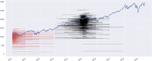
Table 1 This table presents a (simplified) preview of one of the four processed datasets.

Index	Date	Features				Additional information					Target
		${\sigma }_{\text{impl}}\sqrt{\tau }$	M	${\delta }_{\text{BS}}$	${\mathcal{V}}_{\text{BS}}$	S0	S1	C0	$r_{\text{onr}}$	CP flag	C1
0	2018/07/02	0.047	1.003	0.531	9.357	100	98.223	2.002	0.01	0	1.130
$⋮$

NOTES: The “Features” columns are used as inputs for the ANN and the linear regressions. The labels ${\sigma }_{\text{impl}}\sqrt{\tau }$ and M denote the square root of total implied variance and moneyness of the option. The labels ${\delta }_{\text{BS}}$ and ${\mathcal{V}}_{\text{BS}}$ are the BS Delta and Vega. The CP flag indicates whether the corresponding option is a call or a put. Prices and sensitivities are all normalized.

Fig. 2 A schematic graph of HedgeNet. The features are transformed into a hedging position by a fully connected feed-forward neural network (FCNN). The additional input is used to compute the value ${\widehat{C}}_1$ of the replicating portfolio.

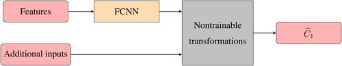
Fig. 3 A detailed schematic presentation of HedgeNet. Recall that $M=S_0/K$ and ${\sigma }_{\text{impl}}\sqrt{\tau }$ are moneyness and square root of total implied variance. “CP flag” is a Boolean flag for the option type; it equals 1 for puts and 0 for calls. Next, S₀ and S₁ are the underlying’s prices at the beginning and end of the hedging period, C₀ denotes the option price at the beginning of the period, and ${\widehat{C}}_1$ denotes the replication value. Finally, $R=1+r_{\text{onr}}\Delta t$ is the risk-free overnight return.

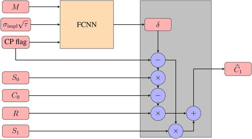
Table 2 Performance of the linear regressions and ANNs on the S&P 500 dataset.

		1 day			2 days
		Calls	Puts	Both	Calls	Puts	Both
	Zero hedge	4.01	4.78	4.54	8.31	9.73	9.29
	BS Delta	0.687	0.655	0.665	1.58	1.54	1.55
$\begin{array}{c}\hfill \\ \hfill \\ \hfill \\ \hfill \\ \hfill \\ \hfill \\ \hfill \\ \hfill \\ \hfill \\ \hfill \\ \hfill \\ \hfill \end{array}\text{Regressions}\{$	Delta-only	–21.3	–14.8	–16.9	–16.3	–12.8	–13.9
	Vega-only	–13.7	–11.7	–12.3	–10.4	–10.1	–10.2
	Gamma-only	–15.5	–10.1	–11.8	–14.5	–11.2	–12.2
	Vanna-only	–12.4	–12.6	–12.5	–10.6	–13.0	–12.2
	Delta-Gamma	–21.6	–14.8	–17.0	–17.1	–13.1	–14.4
	Delta-Vega	– 21.4	– 14.9	– 17.0	– 16.4	– 12.8	– 13.9
	Delta-Vanna	–22.6	–16.6	–18.5	–17.7	–15.4	–16.1
	Delta-Vega-Gamma	–21.5	–14.8	–17.0	–16.8	–13.5	–14.5
	Delta-Vega-Vanna	–23.0	–16.6	–18.7	–18.1	–15.4	–16.2
	Delta-Gamma-Vanna	–22.6	–16.6	–18.5	–17.7	–15.2	–16.0
	Delta-Vega-Gamma-Vanna	–22.9	–16.4	–18.5	–17.4	–14.9	–15.7
	Hull-White	–23.1	–16.9	–18.9	–17.8	–14.5	–15.5
	Relaxed Hull-White	–23.2	–16.9	–18.9	–18.3	–14.6	–15.8
$\begin{array}{c}\hfill \\ \hfill \end{array}\text{ANNs}\{$	$M;{\sigma }_{\text{impl}}\sqrt{\tau }$	–22.3	–15.6	–17.7	–17.1	–10.9	–12.8
	${\Delta }_{\text{BS}};{\mathcal{V}}_{\text{BS}};\tau$	–23.4	–16.9	–18.9	–18.6	–12.9	–14.7
	${\Delta }_{\text{BS}};{\mathcal{V}}_{\text{BS}};{\text{Va}}_{\text{BS}};\tau$	–21.9	–14.4	–16.8	–12.5	–12.9	–12.8

NOTES: The hedging periods $\Delta t$ are here either one day or two days. The columns “Both” are the weighted average of the “Puts” and “Calls” columns. The row “Zero hedge” corresponds to the MSHE when δ = 0 is chosen; that is, the mean squared changes in the option prices. The values in the top two rows are multiplied by 100 to improve readability. The regression and ANN rows correspond to the various statistical models including HedgeNet with three different feature sets. For these two sets of rows, the numbers are reported as relative improvements in MSHE over using the BS Delta, that is, Equation (9)(9) $$\frac{\text{MSHE}({\delta }_{*})-\text{MSHE}({\delta }_{\text{BS}})}{\text{MSHE}({\delta }_{\text{BS}})},$$(9) . Numbers in bold represent the largest outperformance (in each column the best one is chosen along with the ones that are within 1% of the best).

Fig. 4 MSHEs of four different statistical models for the hedging ratio across all 14 time windows in the S&P 500 dataset, for the one-day (left) and two-day (right) hedging period. The in-sample sets for periods 7 and 12 range from 2013 to the first half of 2015 and the second half of 2015 to 2017, respectively. The test data for the 7th time window fall exactly in the 2015–16 selloff. The test data for the 12th time window contain the first week of February 2018, where the S&P 500 experienced a 10% drop; see also Figure 1.

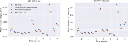
Fig. 5 The coefficients in the Delta-Vega-Vanna regression for each of the 14 time windows in the S&P 500 dataset. The top and bottom of each line segment are the point estimate plus/minus two standard errors. These numbers correspond to the one-day hedging period. The coefficient plots for the two-day hedging periods (not displayed here) look very similar; in particular, the Vanna coefficients for calls are again stable. However, the Vanna coefficients for puts and the Vega coefficients for calls and puts are slightly more fluctuating.

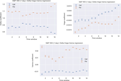
Table 3 Performance of the benchmarks and ANNs on the Euro Stoxx 50 dataset, when the in-sample and out-of-sample are split into one time window.

		1 hr			1 day			2 days
		Calls	Puts	Both	Calls	Puts	Both	Calls	Puts	Both
	Zero hedge	0.431	1.02	0.756	4.28	10.2	7.47	8.20	24.26	17.4
	BS Delta	0.109	0.214	0.167	1.19	1.99	1.62	2.97	4.20	3.67
$\begin{array}{c}\hfill \\ \hfill \\ \hfill \\ \hfill \\ \hfill \\ \hfill \\ \hfill \\ \hfill \\ \hfill \\ \hfill \\ \hfill \\ \hfill \end{array}\text{Regressions}\{$	Delta-only	–18.9	–11.4	–13.6	–21.7	–12.2	–15.4	–36.0	–10.7	–19.5
	Vega-only	–25.3	–13.8	–17.2	–23.4	–16.0	–18.5	–35.2	–16.2	–22.8
	Gamma-only	–0.62	–1.29	–1.10	–15.7	–4.64	–8.37	–32.7	–4.62	–14.4
	Vanna-only	–16.1	–5.18	–8.35	–17.1	–12.6	–14.1	–26.9	–16.9	–20.4
	Delta-Gamma	–18.0	–14.5	–15.5	–20.5	–12.7	–15.4	–33.5	–6.89	–16.1
	Delta-Vega	– 23.9	– 13.7	– 16.7	– 22.7	– 15.4	– 17.9	– 36.9	– 15.3	– 22.8
	Delta-Vanna	–20.8	–11.4	–14.1	–19.2	–14.8	–16.3	–34.9	–17.2	–23.4
	Delta-Vega-Gamma	–21.6	–15.2	–17.0	–20.7	–15.4	–17.2	–34.4	–13.5	–20.8
	Delta-Vega-Vanna	–23.6	–13.7	–16.6	–19.6	–16.7	–17.7	–35.1	–18.5	–24.2
	Delta-Gamma-Vanna	–23.1	–15.5	–17.7	–20.2	–17.9	–18.7	–33.8	–17.7	–23.3
	Delta-Vega-Gamma-Vanna	–23.3	–15.6	–17.8	–20.1	–18.0	–18.7	–34.4	–18.2	–23.9
	Hull-White	–20.0	–12.5	–14.7	–20.7	–14.3	–16.4	–36.1	–13.3	–21.2
	Hull-White-relaxed	–20.3	–12.6	–14.8	–20.6	–14.2	–16.4	–36.1	–12.7	–20.8
$\begin{array}{c}\hfill \\ \hfill \end{array}\text{ANNs}\{$	$M;{\sigma }_{\text{impl}}\sqrt{\tau }$	–17.6	–15.7	–16.3	–8.96	–3.3	–5.21	–27.4	11.3	–2.12
	${\Delta }_{\text{BS}};{\mathcal{V}}_{\text{BS}};\tau$	–16.1	–6.08	–9.01	–19.0	–6.83	–10.9	–25.6	–3.6	–11.2
	${\Delta }_{\text{BS}};{\mathcal{V}}_{\text{BS}};\mathrm{V}{a}_{\text{BS}};\tau$	–25.0	–13.3	–16.7	–18.8	–10.1	–13.1	–29.2	–6.96	–14.7

NOTE: We refer to the caption of Table 2 for an explanation.

Table 4 Coefficients of Delta-Vega-Gamma-Vanna regression for each sensitivity on the Euro Stoxx 50 dataset.

	1 hour		1 day		2 days
	Calls	Puts	Calls	Puts	Calls	Puts
Delta	0.944 ± 0.002	1.134 ± 0.002	0.755 ± 0.003	1.056 ± 0.003	0.821 ± 0.004	1.021 ± 0.003
Vega	$-0.002\pm 0.000$	0.000 ± 0.000	$-0.001\pm 0.000$	$-0.002\pm 0.000$	$-0.001\pm 0.000$	$-0.002\pm 0.000$
Gamma	$-0.021\pm 0.004$	0.213 ± 0.003	$0.226\pm 0.008$	0.393 ± 0.006	0.109 ± 0.010	$0.417\pm 0.008$
Vanna	$-0.010\pm 0.000$	0.014 ± 0.000	0.004 ± 0.000	0.029 ± 0.000	0.003 ± 0.000	0.025 ± 0.000

NOTES: Coefficients are presented for calls and puts separately. Each cell shows the coefficient and its standard error.

Table 5 Performance of the “fixed” hedging strategy on the S&P 500 and Euro Stoxx 50 datasets.

	1 hour			1 day			2 days
	Calls	Puts	Both	Calls	Puts	Both	Calls	Puts	Both
S&P 500	–	–	–	–18.6	–13.1	–14.8	–15.0	–11.4	–12.6
Euro Stoxx 50	–15.4	–10.3	–11.8	–15.4	–12.7	–13.6	–23.7	–16.6	–19.0

NOTES: In the “fixed” hedges strategy, calls (puts) are hedged by $0.9*{\delta }_{\text{BS}}$ ($1.1*{\delta }_{\text{BS}}$). See the caption of Table 2 for further explanations.