Optimal Shrinkage-Based Portfolio Selection in High Dimensions

Figures & data

Fig. 1 Estimated optimal shrinkage intensities for ${\mathbf{S}}_n^{*}$ and ${\mathbf{S}}_n^{+}$(MP) as function of concentration ratio c > 1 and dimension p = 300.

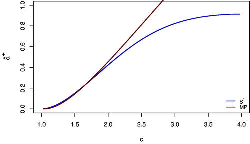
Fig. 2 Estimated optimal shrinkage intensities for ${\mathbf{S}}_n^{*}$ and ${\mathbf{S}}_n^{+}$(MP) as function of dimension p for c = 1.5 (left) and c = 2 (right).

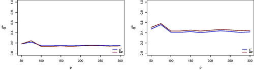
Fig. 3 The asymptotic optimal shrinkage intensity as a function of c for the calibration criteria (i)-(ii) from Proposition 2.1 (left to right).

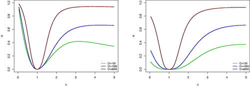
Fig. 4 The relative losses for the portfolios based on the optimal shrinkage estimator, the traditional estimator and the equally weighted portfolio as a function of c for the calibration criteria (i)-(ii) from Proposition 2.1 (left to right). The dimension is set to p = 100 and the condition index is set to 1000.

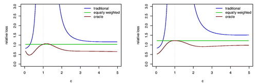
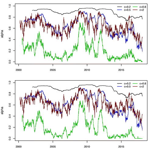
Fig. 5 The relative losses for the portfolios based in the optimal shrinkage estimator, the traditional estimator and the equally weighted portfolio as a function of the dimension p for $c=$ 0.2 (top left), 0.5 (top right), 0.8 (bottom left), 2 (bottom right). The condition index is set to 1000 and the mean-variance calibration criteria is used.

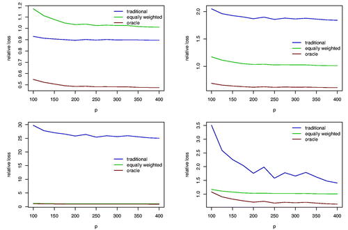
Table 1 Performance of traditional, bona-fide, the benchmark portfolios (LWQuEST— Ledoit and Wolf 2017b, LWAnalytical— Ledoit and Wolf 2020, KZ - Kan and Zhou 2007) and the target portfolios for the mean-variance calibration criteria.

						CE						SR						VaR						ES
						Average		Median				Average			Median			$\alpha =0.05$		$\alpha =0.01$				$\alpha =0.05$		$\alpha =0.01$
$\mathbf{c}=0.2$		trad				–0.84840		–0.84795				0.10033			0.10041			–0.88181		–1.43362				–1.27802		–2.01774
		trad ridge				–0.85096		–0.85028				0.10066			0.1006			–0.88193		–1.43891				–1.28130		–2.02313
		LWQuEST				–0.96539		–0.96509				0.10310			0.10288			–0.93884		–1.52905				–1.35071		–2.10094
		LWAnalytical				–0.79142		–0.79179				0.10141			0.10151			–0.8544		–1.37885				–1.24301		–1.97136
Equally weighted target
		bona fide				–0.80701		–0.80578				0.10125			0.10137			–0.85637		–1.41141				–1.25832		–2.00392
		bona fide ridge				–0.80303		–0.80305				0.10124			0.10136			–0.85485		–1.39997				–1.25366		–1.99908
		target				–1.47973		–1.47978				0.05178			0.05183			–1.35819		–2.17993				–1.90944		–2.91308
		KZ				–0.73868		–0.73831				0.10204			0.10195			–0.81524		–1.33615				–1.20824		–1.94859
Equal correlation target
		bona fide				–0.86149		–0.86029				0.09785			0.09803			–0.90268		–1.48278				–1.30966		–2.06512
		bona fide ridge				–0.86011		–0.85989				0.09773			0.09788			–0.90141		–1.48209				–1.30729		–2.06240
		target				–2.13972		–2.14348				0.05303			0.05291			–1.46652		–2.71956				–2.21071		–3.41674
		KZ				–0.93578		–0.93437				0.09170			0.09159			–0.94118		–1.63936				–1.40500		–2.14364
Fama-French target
		bona fide				–0.85595		–0.85551				0.09504			0.09433			–0.89107		–1.45683				–1.29601		–2.04557
		bona fide ridge				–0.8524		–0.85234				0.09552			0.09556			–0.88859		–1.45891				–1.29374		–2.04100
		target				–2.27656		–2.27951				0.03522			0.03529			–1.44902		–2.83263				–2.21467		–3.40873
		KZ				–0.89766		–0.89748				0.08611			0.08562			–0.89600		–1.58344				–1.34739		–2.09784
$\mathbf{c}=0.5$		trad				–1.56794		–1.56702				0.04112			0.04158			–1.25759		–1.97710				–1.74511		–2.60700
		trad ridge				–1.47446		–1.47309				0.04468			0.04461			–1.2158		–1.90656				–1.68947		–2.53159
		LWQuEST				–3.28708		–3.28730				0.02557			0.02559			–1.85906		–2.93786				–2.56534		–3.68434
		LWAnalytical				–0.86718		–0.86687				0.06531			0.06548			–0.89736		–1.50835				–1.31493		–2.09438
Equally weighted target
		bona fide				–1.02898		–1.02829				0.05067			0.05098			–1.00189		–1.67912				–1.458300		–2.30347
		bona fide ridge				–0.99158		–0.9911				0.05342			0.05347			–0.98209		–1.65375				–1.43523		–2.27809
		target				–1.47854		–1.47831				0.05167			0.05170			–1.35780		–2.18133				–1.90904		–2.91312
		KZ				–0.93245		–0.93159				0.05903			0.05973			–0.95118		–1.50578				–1.34866		–2.10714
Equal correlation target
		bona fide				–1.18004		–1.17898				0.05198			0.05215			–1.10187		–1.82427				–1.59237		–2.44481
		bona fide ridge				–1.15576		–1.15526				0.05312			0.05308			–1.09212		–1.81848				–1.58300		–2.43487
		target				–1.81699		–1.81663				0.04036			0.04029			–1.40816		–2.42265				–2.10357		–3.33301
		KZ				–1.01288		–1.01141				0.05760			0.05770			–1.01531		–1.57685				–1.41783		–2.14790
Fama-French target
		bona fide				–1.22574		–1.22594				0.04963			0.04973			–1.11090		–1.75940				–1.57373		–2.42489
		bona fide ridge				–1.19113		–1.19039				0.05083			0.05064			–1.09567		–1.73454				–1.55387		–2.40117
		target				–1.93351		–1.9336				0.04278			0.04265			–1.40284		–2.48907				–1.99845		–2.92676
		KZ				–1.01496		–1.01416				0.05761			0.05782			–1.00263		–1.55246				–1.40187		–2.16018
$\mathbf{c}=0.8$		trad				–11.10781		–11.07733				0.04031			0.03992			–3.35917		–5.40548				–4.66218		–6.70938
		trad ridge				–5.60256		–5.59981				0.04942			0.04921			–2.40138		–3.8217				–3.29866		–4.71741
		LWQuEST				–18.80892		–18.81717				0.03520			0.03521			–4.51683		–6.92530				–6.05810		–8.35046
		LWAnalytical				–0.98453		–0.98438				0.08988			0.08999			–0.98071		–1.61591				–1.42389		–2.24346
Equally weighted target
		bona fide				–1.40577		–1.40584				0.05118			0.05134			–1.29895		–2.07527				1.83362		–2.79312
		bona fide ridge				–1.31635		–1.31596				0.05238			0.05235			–1.28390		–2.02482				–1.79171		–2.74021
		target				–1.48023		–1.47918				0.05170			0.05171			–1.35865		–2.18186				–1.91045		–2.9148
		KZ				–2.03472		–2.03185				0.06359			0.06288			–1.40796		–2.25191				–1.97686		–2.94533
Equal correlation target
		bona fide				–1.60399		–1.60241				0.04978			0.04984			–1.29237		–2.39802				–1.98752		–3.17541
		bona fide ridge				–1.55829		–1.55768				0.05013			0.05005			–1.26800		–2.35739				–1.96495		–3.16411
		target				–1.68942		–1.68949				0.04453			0.04452			–1.3124		–2.45543				–2.05351		–3.35801
		KZ				–1.96623		–1.96299				0.06550			0.06522			–1.37667		–2.20379				–1.93809		–2.91761
Fama-French target
			bona fide		–1.79593				–1.79528		0.04740			0.04760			–1.39084				–2.26699		–1.94795			–2.84830
			bona fide ridge		–1.69800				–1.6972		0.04796			0.04793			–1.34454				–2.23851		–1.90270			–2.78836
			target		–1.83876				–1.83798		0.04355			0.04365			–1.37985				–2.41411		–1.98305			–2.94513
			KZ		–2.06935				–2.07129		0.06506			0.06515			–1.41329				–2.27824		–1.98427			–2.95639
$\mathbf{c}=2.0$			trad		–2.12939				–2.13080		0.06414			0.06427			–1.44683				–2.38186		–2.07522			–3.18270
			trad ridge		–2.05179				–2.05106		0.06509			0.06514			–1.42082				–2.34175		–2.03791			–3.12989
			LWQuEST		–59.03298				–58.99561		0.00629			0.00618			–7.9549				–12.68863		–10.94189			–15.31889
			LWAnalytical		–1.50503				–1.50439		0.06355			0.06375			–1.26581				–1.95316		–1.7726			–2.69539
Equally weighted target
	bona fide			–1.22550			–1.22474			0.05904			0.05907			–1.18681			–1.99190			–1.72914			–2.75302
	bona fide ridge			–1.30872			–1.30891			0.06790			0.06782			–1.14901			–1.94775			–1.70477			–2.73827
	target			–1.47869			–1.47779			0.05175			0.05176			–1.35801			–2.17908			–1.90898			–2.91238
Equal correlation target
	bona fide			–1.22592			–1.22761			0.07282			0.07288			–1.09681			–2.09756			–1.74639			–2.91502
	bona fide ridge			–1.24075			–1.23914			0.07872			0.07873			–1.10084			–1.93814			–1.67112			–2.70638
	target			–1.32850			–1.32805			0.07020			0.07020			–1.13496			–2.16850			–1.83174			–3.08545
Fama-French target
	bona fide			–1.44490			–1.44438			0.05890			0.05867			–1.22790			–2.09709			–1.75667			–2.65269
	bona fide ridge			–1.42024			–1.41913			0.06947			0.06922			–1.19613			–1.96825			–1.72476			–2.66945
	target			–1.62084			–1.62093			0.05377			0.05360			–1.29152			–2.34075			–1.86625			–2.83814

NOTE: The performance measures are averaged over 1000 random portfolios of size 300. The trading period consists of 1000 days preceding March 23, 2018 and the risk aversion is set to 5. The average values are based on trimmed mean with 10% of extreme values being dropped. The best strategies for every criteria and every values of c are highlighted in bold.

Table 2 Performance of traditional, bona-fide, the benchmark portfolios (LWQuEST - Ledoit and Wolf 2017b, LWAnalytical - Ledoit and Wolf 2020, KZ - Kan and Zhou 2007) and the target portfolios for the minimum variance calibration criteria.

					CE					SR							VaR						ES
					Average			Median		Average				Median			$\alpha =0.05$			$\alpha =0.01$			$\alpha =0.05$			$\alpha =0.01$
$\mathbf{c}=0.2$		trad			–0.85309			–0.85231		0.10035				0.10057			–0.88250			–1.44210			–1.28383			–2.02584
		trad ridge			–0.84923			–0.84889		0.09923				0.09909			–0.88174			–1.43823			–1.27883			–2.01864
		LWQuEST			–0.96554			–0.96474		0.10343				0.10359			–0.93948			–1.52539			–1.35090			–2.10343
		LWAnalytical			–0.79114			–0.79048		0.1014				0.10161			–0.85381			–1.38047			–1.24188			–1.96952
Equally weighted target
		bona fide			–0.81308			–0.81284		0.10123				0.10150			–0.85908			–1.41182			–1.26178			–2.0085
		bona fide ridge			–0.80998			–0.81034		0.10012				0.10001			–0.85828			–1.40687			–1.25735			–2.00243
		target			–1.47805			–1.47784		0.05169				0.05168			–1.35704			–2.17938			–1.90829			–2.91097
		KZ			–0.73828			–0.73822		0.10187				0.10195			–0.81400			–1.33608			–1.20828			–1.95301
Equal correlation target
		bona fide			–0.85773			–0.85717		0.09806				0.09785			–0.89740			–1.47224			–1.30236			–2.05662
		bona fide ridge			–0.85262			–0.85171		0.09803				0.0981			–0.89563			–1.46898			–1.29994			–2.05272
		target			–2.13255			–2.12898		0.05319				0.05312			–1.46343			–2.71591			–2.20532			–3.40780
		KZ			–0.93731			–0.93588		0.09141				0.09120			–0.94052			–1.63821			–1.40403			–2.14399
Fama-French target
		bona fide			–0.85149			–0.85077		0.09663				0.09677			–0.88750			–1.45256			–1.29064			–2.03126
		bona fide ridge			–0.84949			–0.84947		0.09629				0.09625			–0.88760			–1.44700			–1.28814			–2.0294
		target			–2.27063			–2.26895		0.03538				0.03543			–1.44480			–2.82390			–2.21059			–3.40190
		KZ			–0.89663			–0.89478		0.08661				0.08659			–0.89534			–1.58062			–1.34627			–2.09320
$\mathbf{c}=0.5$		trad			–1.56971			–1.57001		0.04173				0.04161			–1.26072			–1.97665			–1.74582			–2.60683
		trad ridge			–1.47585			–1.4756		0.04465				0.0444			–1.21598			–1.90785			–1.69053			–2.54353
		LWQuEST			–3.28833			–3.29027		0.02581				0.02608			–1.86558			–2.93777			–2.56735			–3.67757
		LWAnalytical			–0.86699			–0.86626		0.0654				0.06526			–0.89816			–1.50838			–1.31504			–2.0954
Equally weighted target
		bona fide			–1.0532			–1.05298		0.05066				0.05048			–1.01036			–1.69687			–1.46966			–2.30812
		bona fide ridge			–1.14637			–1.14571		0.05275				0.05322			–1.08067			–1.78718			–1.56281			–2.41015
		target			–1.48082			–1.48066		0.05171				0.05172			–1.35847			–2.18138			–1.91024			–2.91449
		KZ			–0.93323			–0.93338		0.05939				0.05941			–0.95222			–1.50541			–1.34938			–2.10436
Equal correlation target
		bona fide			–1.17591			–1.17430		0.05196				0.05184			–1.09485			–1.80109			–1.57693			–2.42242
		bona fide ridge			–1.14637			–1.14571		0.05275				0.05322			–1.08067			–1.78718			–1.56281			–2.41015
		target			–1.80886			–1.80920		0.04010				0.04001			–1.40596			–2.41696			–2.09826			–3.32139
		KZ			–1.01397			–1.01394		0.05762				0.05790			–1.01524			–1.58062			–1.41661			–2.14494
Fama-French target
	bona fide		–1.22924				–1.22845		0.04980				0.05017			–1.11019			–1.75950			–1.56925			–2.41742
	bona fide ridge		–1.18967				–1.18982		0.05057				0.05064			–1.09012			–1.72857			–1.54528			–2.39013
	target		–1.93623				–1.93641		0.04259				0.04257			–1.40372			–2.49587			–2.00108			–2.93538
	KZ		–1.01377				–1.01328		0.05759				0.05765			–1.00204			–1.55270			–1.40064			–2.15907
$\mathbf{c}=0.8$	trad		–11.1587				–11.12847		0.03821				0.03725			–3.3777			–5.43327			–4.67808			–6.73814
	trad ridge		–5.59307				–5.5935		0.05126				0.05138			–2.39789			–3.80057			–3.28431			–4.69414
	LWQuEST		–18.84221				–18.84773		0.03577				0.03624			–4.50978			–6.96099			–6.06441			–8.39818
	LWAnalytical		–0.98496				–0.98436		0.08942				0.08955			–0.98112			–1.61597			–1.42344			–2.2402
Equally weighted target
	bona fide			–1.43449		–1.43529					0.05084	0.0503			–1.30108			–2.08832			–1.83907			–2.79121
	bona fide ridge			–1.30591		–1.30557					0.05487	0.05487			–1.26708			–1.99403			–1.77592			–2.71366
	target			–1.47821		–1.47811					0.05168	0.05169			–1.35667			–2.18041			–1.90876			–2.91209
	KZ			–2.03415		–2.03269					0.06235	0.06256			–1.41138			–2.25474			–1.97862			–2.94248
Equal correlation target
	bona fide			–1.60982		–1.60906					0.05073	0.05031			–1.29875			–2.39866			–1.98344			–3.15048
	bona fide ridge			–1.53174		–1.52924					0.05174	0.05171			–1.26259			–2.35322			–1.94643			–3.11905
	target			–1.68850		–1.68914					0.04481	0.04491			–1.31139			–2.45712			–2.05434			–3.36065
	KZ			–1.96089		–1.95878					0.06499	0.06450			–1.37460			–2.19955			–1.93337			–2.90941
Fama-French target
	bona fide			–1.82002		–1.82289					0.04739	0.04775			–1.40332			–2.25988			–1.95652			–2.86186
	bona fide ridge			–1.6811		–1.67987					0.04983	0.04971			–1.34377			–2.20183			–1.89093			–2.77691
	target			–1.83460		–1.83658					0.04329	0.0432			–1.37616			–2.40806			–1.98023			–2.93814
	KZ			–2.07064		–2.06718					0.06476	0.06399			–1.41264			–2.27641			–1.98342			–2.96439
$\mathbf{c}=2.0$	trad			–2.12727		–2.12819					0.06405	0.0641			–1.44373			–2.38377			–2.07218			–3.17711
	trad ridge			–2.06068		–2.05893					0.06518	0.06514			–1.4236			–2.34051			–2.04197			–3.13703
	LWQuEST			–58.92062		–58.87816					0.00574	0.00587			–7.96587			–12.64654			–10.9261			–15.29078
	LWAnalytical			–1.50775		–1.50743					0.064	0.06383			–1.26662			–1.9523			–1.77553			–2.70126
Equally weighted target
	bona fide			–1.45575		–1.45568					0.05220	0.05226			–1.34997			–2.15551			–1.89422			–2.89468
	bona fide ridge			–1.2937		–1.29318					0.06757	0.06793			–1.14349			–1.94082			–1.69787			–2.73005
	target			–1.4788		–1.47899					0.05174	0.05177			–1.35821			–2.17967			–1.90906			–2.91205
Equal correlation target
	bona fide			–1.31924		–1.32062					0.07073	0.07077			–1.13066			–2.15773			–1.82514			–3.07313
	bona fide ridge			–1.22331		–1.22256					0.07853	0.07837			–1.09087			–1.93172			–1.66227			–2.69818
	target			–1.32790		–1.32922					0.07046	0.07044			–1.13449			–2.16647			–1.83165			–3.08673
Fama-French target
	bona fide			–1.60447		–1.60370					0.05413	0.05423			–1.28581			–2.32282			–1.85587			–2.82089
	bona fide ridge			–1.41559		–1.41478					0.06915	0.06884			–1.19404			–1.97205			–1.72228			–2.66687
	target			–1.61993		–1.62003					0.05373	0.05383			–1.29209			–2.33933			–1.86513			–2.83576

NOTE: The performance measures are averaged over 1000 random portfolios of size 300. The trading period consists of 1000 days preceding March 23, 2018 and the risk aversion is set to 5. The average values are based on trimmed mean with 10% of extreme values being dropped. The best strategies for every criteria and every values of c are highlighted in bold.

Fig. 6 The bona-fide shrinkage intensities for the first 100 assets (alphabetic order) using the equally weighted target portfolio and the mean-variance calibration for c = 0.2, 0.5, 0.8 and 2. Above - bona fide, below - bona fide ridge (see formula (2.33)).

Kan, R., and Zhou, G. (2007), “Optimal Portfolio Choice with Parameter Uncertainty,” The Journal of Financial and Quantitative Analysis, 42, 621–656. DOI: 10.1017/S0022109000004129.

 Web of Science ®Google Scholar