Bayesian Nonparametric Panel Markov-Switching GARCH Models

Figures & data

Figure 1: Top panel: rolling window estimates of the log-volatility (left) and log-kurtosis (right) for the S&P100’s constituents from 6th January 2000 to 3rd October 2020 (30 weeks window). Vertical bars indicate three reference dates: 6th July 2002, 23rd August 2008 and 22nd February 2020. Bottom panel: cross-sectional distribution of the log-volatility (left) and log-kurtosis (right) in three reference dates.

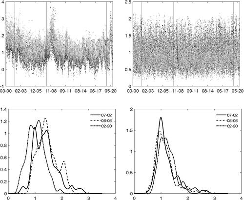
Figure 2: DAG of the Bayesian nonparametric panel MSGARCH model. It exhibits the hierarchical structure of the observations ${\mathbf{y}}_t=(y_{1t},\dots ,y_{Nt})$ (boxes), the latent state variables ${\mathbf{s}}_t=(s_{1t},\dots ,s_{Nt})$ (gray circles), the parameters of the transition probability matrix $P_i=({\mathbf{p}}_{i,1},\dots ,{\mathbf{p}}_{i,K})$, ${\theta }_i=({\mu }_i,{\gamma }_i,{\alpha }_i,{\beta }_i)$, the hyperparameters of the first stage $R=({\mathbf{r}}_1,\dots ,{\mathbf{r}}_K)$, ${\tilde{\theta }}_i^{\ast }=({\tilde{\mu }}_i^{*},{\tilde{\gamma }}_i^{*},{\tilde{\alpha }}_i^{*},{\tilde{\beta }}_i^{*})$ and of the second stage G (white circles). The directed arrows show the conditional independence structure of the model.

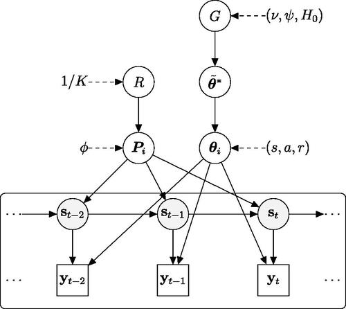
Figure 3: The posterior co-clustering matrix in regime 1 (left) and 2 (right) for expected returns (top) and volatility (bottom) identification constraints. In each block, gray shades represent the sector membership of the assets.

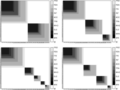
Figure 4: Price-to-Earning for the assets in clusters of regime 1 (left) and of regime 2 (right), constraint on expected returns (top panel). Logarithm of implied volatility for the assets in clusters of regime 1 (left) and of regime 2 (right), constraint on volatility (bottom panel).

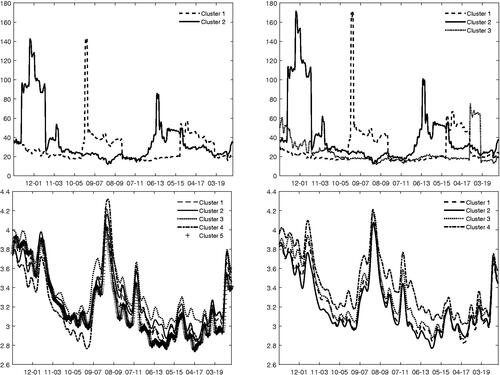
Table 1: Out-of-sample evaluation. RMSE and CRPS.

Models	RMSE
	Full period	pre-COVID period	COVID  period
BNP-MSGARCH-$\mu$	3.829	3.047	7.156
BNP-MSGARCH-$\gamma$	3.826	3.045	7.152
BNP-GARCH	3.823	3.041	7.151
GARCH	3.830	3.042	7.180
Models	CRPS
	Full period	pre-COVID period	COVID period
BNP-MSGARCH-$\mu$	1.931	1.677	3.867
BNP-MSGARCH-$\gamma$	1.927	1.674	3.865
BNP-GARCH	2.026	1.783	3.890
GARCH	2.026	1.777	3.913
Models	SR
	Full period	pre-COVID period	COVID period
BNP-MSGARCH-$\mu$	0.124	0.127	0.107
BNP-MSGARCH-$\gamma$	0.111	0.114	0.088
BNP-GARCH	0.103	0.104	0.095
GARCH	0.090	0.079	0.088

NOTES: BNP-MSGARCH-$\mu$ and BNP-MSGARCH-$\gamma$ are the Bayesian nonparametric panel Markov-Switching models with restrictions on expected returns and on volatility, respectively; GARCH is the standard GARCH model; BNP-GARCH is the Bayesian nonparametric GARCH model without regime changes. RMSE, CRPS, and SR are the averages of the root mean square error, the continuous ranked probability score, and the Sharpe ratio, respectively. The COVID period starts in early February 2020, see Centers for Disease Control and Prevention (CDC)).